Page 55 - ITU Journal Future and evolving technologies Volume 2 (2021), Issue 5 – Internet of Everything

ITU Journal on Future and Evolving Technologies, Volume 2 (2021), Issue 5

0.2 0.2 0.2

0.1
Amplitude (Volts) -0.1 0 Amplitude (Volts) -0.1 0 Amplitude (Volts) -0.1 0
0.1
0.1

-0.2 -0.2 -0.2
0 0.05 0.1 0.15 0.2 0.25 0 0.05 0.1 0.15 0.2 0.25 0 0.05 0.1 0.15 0.2 0.25
Time (ms) Time (ms) Time (ms)

10 10 10 0
8 8 8 −20
Frequency (GHz) 6 4 Frequency (GHz) 6 4 requency (GHz) 6 4 −40 Density (dB/Hz)

−60
2 2 F 2 −80
−100
0 0 0
0 0.05 0.1 0.15 0.2 0.25 0 0.05 0.1 0.15 0.2 0.25 0 0.05 0.1 0.15 0.2 0.25
Time (ms) Time (ms) Time (ms)
(a) (b) (c)

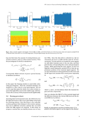
Fig. 3 – Noisy controller signal of a DJI Inspire 1 Pro for different SNRs: a) 30 dB, b) 15 dB, and c) 0 dB. Base noise in lab environment is around 30 dB.
As SNR decreases, distortion occurs for both image types. All spectrogram images have the same density color scale.

hop size that tunes the amount of overlap between con‑ low SNRs. Since the data [26] is collected in a lab en‑
secutive windows, and [ ] is the window function. Then vironment, the noise is stable and the same for all mea‑
the periodogram of a block is calculated as surements. To train and test our models for noisy signals,
we add white Gaussian noise to the raw data, and then
1
, ( ) = | , ( )| 2 (2) generate the corresponding time‑series and spectrogram

images. While generating the noisy signals, we irst use
1 −1 Higuchi’s fractal dimension method [35] to ind the ap‑
= ∣∑ [ ] −2j / ∣ .

proximate position of the transient signal segment. We
=0
use this information to distinguish between the noise and
Consequently, Welch estimate of power spectral density the RF signal and calculate their actual power separately
is calculated as follows as
∑ | [ ]| 2
=0
1 −1 noise [dB] = 10 × log 10 ( ) , (4)
̂ = ∑ , ( ). (3)

=0 and

In this paper the Hanning window is used while calcu‑ ⎛ ∑ | [ ]| 2 ⎞
lating preiodograms. Then the calculated densities are signal [dB] = 10 × log 10 ⎜ = ⎟ , (5)
−
mapped to a color scale to create spectrograms. We use ⎝ ⎠
a color map that spans the whole color space evenly, i.e., where and are the indexes where the transient be‑

passes through all the colors in the visible range, which in‑ gins and ends, respectively.
creases the accuracy of the proposed model signi icantly.
Next, we calculate the SNR (Γ) of the received signal and
3.2 Noising procedure the difference between the current SNR level and the de‑
sired SNR level as follows:
Assuming ixed environmental noise, the SNR level of an
RF signal decreases as the source gets farther away from Γ signal [dB] = signal − noise , (6)
the receiving antenna. Since the drone or the controller and
position and hence their distance to the receiver antenna ΔΓ [dB] = Γ − Γ . (7)
may vary in different scenarios, systems that can work signal desired
under low SNR regimes are required. In this study, we Finally, an appropriate amount of random noise [ ] is
propose a method that can identify drones even at very added to the whole signal to set the signal to the desired

© International Telecommunication Union, 2021 43