Page 57 - ITU Journal Future and evolving technologies Volume 2 (2021), Issue 5 – Internet of Everything

ITU Journal on Future and Evolving Technologies, Volume 2 (2021), Issue 5

the truncation process is essentially a denoising proce‑ 4.3 Training and testing CNN models
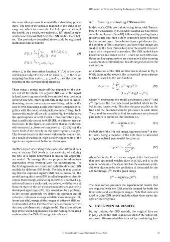
dure. The rest of the signal is mapped to the same color In this work, CNNs are trained using Keras with Tensor‑
range set, which increases the level of representation of low at the backend. In the models created, we have three
the details. As a result, non‑noise (i.e., RF) signal compo‑ convolution layers (Conv2D) followed by pooling layers
nents come forward that help the CNN models learn bet‑ (MaxPool2D) and then a fully connected layer followed
ter. The procedure described above could be explained by the output layer. Convolution layers get deeper (i.e.,
mathematically as follows:
the number of ilters increase), and size of the images get
smaller as the data travels deep into the model, in accor‑
, if [ , ] ≤ dance with the general convention. The CNN models have

′
[ , ] −→ { , (9)
[ , ], else been trained and tested with 3 ∶ 1 ratio for each UAV class.
Optimum hyperparameters are determined after running

′
[ , ] −→ , , , , , , a vast amount of simulations. Results are presented in the
next section.
′
where is the truncation function, [ , ] is the trun‑ An illustration of the CNN architecture is shown in Fig. 5.

cated signal subject to the cut‑off value , is the color While training the models, the categorical cross‑entropy

mapping function, and , , , , and , are the color in‑ function is used as the loss function
tensities in the corresponding channels.
1
( )
ℒ( ) = − ∑ [ ( ) log( ̂ )+ (10)
There exists a critical trade‑off that depends on the cho‑ =1
( )
( )
sen cut‑off threshold. For a given SNR level of the signal (1 − ) log(1 − ̂ )],
in hand, spectrograms should be truncated at an optimum
level for that SNR. More speci ically, in the case of under‑ where represents the model parameters, and ( ) and
̂
denoising, excess noise causes over itting, while in the ( ) represent the true labels and predicted labels for the
case of over‑denoising, useful information is wiped out to‑ ‑th image, respectively. This function gets smaller as the
gether with the noise, which yields to under itting. To il‑ true and the predicted results get closer to each other.
lustrate this trade‑off, we will consider Fig. 4 which shows The aim of the model is to ind the optimum set of model
the spectrograms of a DJI Inspire 1 Pro controller signal, parameters to minimize this function, i.e.,
that is arti icially noised to 0 dB SNR, at different trunca‑ ̂
tion levels. In this igure, it is observed that as the thresh‑ = argmin ℒ( ). (11)

old increases (i.e., from no truncation to −20 dB/Hz), the
lower limit of the density on the spectrograms changes. Probability of the ‑th test image, expressed as x ( ) in vec‑
This lowest density is the lowest value in the domain set. tor form, being a member of the ‑th class is calculated
As a result of truncation, high density components of the using normalized exponential function as:
signals are represented better on the images.
( )
̂
( )
(x ) = , (12)

Another aspect of creating CNN models for different data ∑ ( )
̂

sets at various SNR levels is the necessity of de ining
the SNR of a signal beforehand to invoke the appropri‑ where ̂v (i) is the × 1 vector output of the inal model
ate model. To manage this, we propose to follow two that uses optimized weights given in ((11)), and is the
approaches while working with the spectrograms. In number of classes. The class that has the maximum prob‑
the irst approach, we create and optimize different CNN ability is chosen to be the prediction of the model for the
models for different SNR levels. The idea is that, assum‑ ‑th test image, ̂ , for the given image
( )
ing that the captured signal’s SNR can be measured, the
model having the closest SNR is called to perform classi i‑ ( ) = argmax (x ). (13)
( )
̂

cation. Even though, calculating the SNR of a received sig‑
nal in real time is a tricky task, we believe, with the help of The next section presents the experimental results that
featured state‑of‑the‑art measurement devices and newly are acquired with the CNN models created for both the
developed algorithms [37], this would not be a problem. time‑series and spectrogram images. Note that data sets
In the second approach, we de ine an optimum cut‑off used to train CNN models include either time‑series im‑
value (i.e., minimum average validation loss among all dif‑ ages or spectrograms.
ferent cut‑offs), merge all the images of different SNR lev‑
els truncated at this level to create a new comprehensive
data set, and then train a single model. The major advan‑ 5. EXPERIMENTAL RESULTS
tageofthissecondapproachisthatitisnolongerrequired During training the CNN models, the original data set
to determine the SNR of the signal in advance. in [26], where the SNR is about 30 dB for the whole set,
was used. We extended this data set by considering four

© International Telecommunication Union, 2021 45