Page 64 - ITU Journal Future and evolving technologies Volume 3 (2022), Issue 2 – Towards vehicular networks in the 6G era

ITU Journal on Future and Evolving Technologies, Volume 3 (2022), Issue 2

5. SIMULATION RESULTS

In this section, we present the simulation setup and verify
our proposed analysis model with simulations to ensure
the correctness. We will give more results for investiga‑
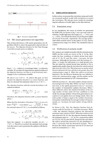
Source Traffic light Destination ting the in luence of traf ic lights on the data delivery.

5.1 Simulation setup
1 2
In our simulations, the traces of vehicles are generated
by SUMO [29]. As shown in Fig. 7, two one‑way roads di‑
vided by a traf ic light have the length of = 1100 and
1
Fig. 7 – Simulation setup by SUMO = 800 . The default durations of red and green lights
2
are 28 and 70 seconds, respectively. The average speed
4.4 TAC‑aware generation rate algorithm
with which vehicles move on the path is 15 m/s, and its
This section introduces a TAC‑aware generation rate Al‑ communication range is 300m. The simulation time is
gorithm (TACA) to select the generation interval time of 1 hour.
the source. The objective function for the Total Average
Cost (TAC) of each cycle is as follows: 5.2 Veri ication of analysis model
Δ + ⋅ ℎ We compare our analytical model with the simulations by
( ) = [ ℎ ]
SUMO, and the results are shown in Fig. 8. In Fig. 8(a),
⋅ ( + 2 ) (2 + 3 ) ⋅ 2 under the four conditions of vehicle arrival time inter‑
= + vals of 15, 20, 25, and 30s; when increases, AoI also
2 ⋅ ⋅ ⋅ 2 increases. Although AoI increases with the increase of ,

2
⋅ 2 − 2 2 + − when is larger, AoI still grows at a small growth rate.
+ + 1 2 (10)
2 ⋅ ⋅ The AoI when the vehicle arrival time interval is 15s is
2
signi icantly smaller than the AoI when the vehicle arrival
Since = ⋅ where is an integer value, is a discrete time interval is 20 or 25s. This is because we set the initial
0
0
variable. To calculate the approximate optimal solution of distance between the two vehicles to be greater than the
the objective function, we relax to be fractional, and communication range . When the vehicle arrival time
0
changes to be a continuous variable. interval is 15s, the distance between the two vehicles is
within the communication range, and the update can be
We aim to ( ). To achieve this goal, we irst transmitted immediately by V2V communications.
present the objective function is a convex function, and
then we calculate the minimum value of ( ). With the increase of , the total number of hops shows a
decreasing trend in Fig. 8(b). Within one hour of simula‑
The objective function with the second derivative is cal‑ tion time, as the update generation interval increases,
culated as follows: the number of transmitted updates decreases. When
2
( ) = 2 (2 + 3 ) ⋅ 1 > 0 (11) takes different values, the standard deviation of the ave‑

rage number of hops under the four conditions is very
2
2 3 small; the average number of hops from generation to re‑
ception of each update does not change much. Since the
Therefore, the objective function with a convex function
total number of hops is equal to the number of transmit‑
about .
ted updates multiplied by the average number of hops per
When the irst derivative of function ( ) is set as 0, update, as increases, the total number of hops will de‑
⋅ . Then
thatis ( ) = 0, weobtain = √ 4 +6 crease.
+2
the minimal value of ( ) is calculated as follows: As shown in Fig. 8(c), the objective function irst de‑
creases with the increase of , and then increases. When
√ + 2 ⋅ √4 + 6 =38s, the objective function achieves the theoretical

= ⋅
⋅ minimum value, which is 155.07. When the vehicle arrival
2
⋅ 2 − 2 2 + − time interval is 20, 25, 30s, the objective function obtains
+ + 1 2 (12) the minimum value at = 47, 46, 46 , respectively, which
2
2

are 141.56, 141.92, and 148.43. Except for the case where
Since the original is a discrete variable, we set = the vehicle arrival time interval is 15s, the simulation re‑
⌊ ⌋⋅ . Therefore, to achieve the minimal total average sults is consistent with the theoretical analysis. This is

cost, the sensor source generates the updates with this in‑ because the vehicle arrival time interval of 15s does not
terval time. meet our assumption ( > 20 ).
52 © International Telecommunication Union, 2022