Page 62 - ITU Journal Future and evolving technologies Volume 3 (2022), Issue 2 – Towards vehicular networks in the 6G era

ITU Journal on Future and Evolving Technologies, Volume 3 (2022), Issue 2

up to peak
Traffic hole
Traffic light layer
steady
V2R V2V V2R
Updates layer 4 3 2 1
drop down Source Destination
Vehicle layer v

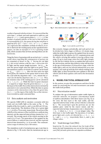
Fig. 3 – Data analysis for AoI by SUMO Fig. 4 – Discretization model of update delivery under traf ic light

number of queued vehicles at time . It is assumed that the age R/v
v
cycle time is ixed, and each approach is split in a red

phase (0 < ≤ ) and a green phase ( < ≤ ). If the V2V

number of queued vehicles at the start of the red phase time
is represented by (0), the queue during the red phase is R
t t ’ t ”
given by [27]: ( ) = (0) + ( ), (0 < ≤ ), where

( ) represents the cumulative arrivals of vehicles. In or‑ Fig. 5 – Cost model for each V2V hop
der to illustrate the waiting queue at the signalized inter‑
this scenario changes periodically, and each period can
section, we take an example of / /1 queueing model
be divided into three stages as follows: (1) steady stage,
[28], which assumes that arrivals and departures are de‑
terministic. while the traf ic light is green, the update from the source
is delivered by the vehicles via V2V communications and
Using the form of queueing with an arrival rate , certain the vehicle carrying this update is moving without stop‑
useful values regarding the consequences of queues can ping; (2) up‑to‑peak stage, when the traf ic light changes
be computed as shown in Fig. 2. During the red light to red, the irst vehicle carries an update that will stop at
( ), the arrival vehicles with the rate wait at the traf‑ the intersection, and the data delivery delay will increase

ic light, and the queue length increases. Let de‑ to the age of information; (3) drop‑down stage, while the
note the queue length when the light turns green. Thus, traf ic light is still red, the vehicles behind that carry new
the maximum number of vehicles in a queue can be found updates, will catch up with the irst vehicle waiting at the
as: = (0) + ⋅ . After the time when the light traf ic light, so they forward the new updates to the irst

turns green, the vehicles in the queue start to move onto vehicle and all these updates will send to the destination
the road with the departure rate . Let denote the ar‑ at once.
rival rate divided by departure rate, i.e. = / . Thus,
the clearance time of the waiting queue can be calculated 4. MODEL FOR TOTAL AVERAGE COST
as: = /(1 − ). While the time to queue clearance

is equal to or larger than the green time (i.e. ≥ ), In this section, we give the assumptions and describe the

the input of the traf ic low at the intersection is termed as model for analyzing the AoI and transmission cost under
saturated or over‑saturated low. While the time to queue the traf ic hole problem.
clearance at the intersection is less than the green time,
4.1 Discretization model
(i.e. < ), the input of the traf ic low at the intersec‑

tion is termed as under‑saturated low. To analyze the age of information under traf ic lights in
vehicular networks, we propose a discretization model
3.3 Data analysis and motivation of uniform distribution with three layers (see Fig. 4) as
fol‑ lows: the irst layer is the road traf ic, and the
We operate SUMO [29] to simulate a scenario with two expected interval time of the arrival vehicles is denoted
roads and one tr ic light as the same as Fig. 1. The
by . The second layer upon the previous one are the
lengths of the two roads ( and ) are 800 and 101 me‑ updates gene‑ rated by the source sensor, and the
1
2
ters, respectively. The duration of the red or green light expected interval time of generation rate is denoted by
( / ) is 28 or 70 seconds, respectively. The arrival of the = ⋅ where ∈ {1, 2, ⋯} is an integer value. The

vehicles at the entrance of the road follows a uniform time 0 0
third layer is the traf ic light. The durations of red light,
interval, and the expected interval time denoted by is 7 green light and a cycle, are denoted by = ⋅ , =
seconds. The average speed of the vehicle moving on the
⋅ and = + , respectively. Here, and are

road ( ) is 15 m/s. The generation of the updates by the
integer values.
source follows a uniform time interval, and the expected
interval time denoted by is 16 seconds. The communi‑ 4.2 Total Average Cost (TAC)
cation range of vehicles ( ) is 100 meters.
Inspired by [7], since the network has the trade‑off be‑
The simulation result of instantaneous age at any time is tween AoI and transmission cost, we set the total average
shown in Fig. 3. We notice that the instantaneous age in cost (TAC) of each cycle to be our objective as follows:
50 © International Telecommunication Union, 2022