Page 32 - ITU Journal Future and evolving technologies Volume 2 (2021), Issue 4 – AI and machine learning solutions in 5G and future networks

ITU Journal on Future and Evolving Technologies, Volume 2 (2021), Issue 4

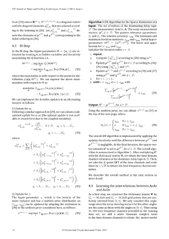
from [29] where D ( ) ∈ ℝ × is a diagonal matrix Algorithm 1 EM Algorithm for the Sparse Estimation of x
( )
with the diagonal elements , that are ordered accord‐ Input: The set of indices of the dominating delay taps:
ing to the indexing in (26). Let ( ) and ( ) de‐ . The measurement matrix: A. The noisy measurement

, , vectors: y , ∈ . The pattern relevance parameters:
note the elements of ( ) and ( ) corresponding to the and . The solution accuracy: . The minimum and

EM
index ordering in (26). maximum iteration numbers: and . Initial hyper‐
min max
(0)
parameters: Θ (0) = { , (0) }. The lower and upper
4.3 M‐Step bounds for : low and upp .
Initialize the iteration index ← 0.
In the M‐step, the hyper‐parameters Θ = { , } are es‐
1: repeat
timated by treating x as hidden variables and iteratively
( ) ( )
maximizing the Q‐function, i.e., 2: Compute { , } according to (28) using .
( ) ( )

( )
Θ ( +1) = arg max (Θ|Θ ) 3: Update and , for ∈ according to (30)‐
Θ ( ) ( )
(31) using { , } and .
= arg max x|y,Θ ( ) [ln (Θ|x, y)] , (32) ( +1) ( +1)
Θ 4: Update and according to (34) and (37)
( ) ( )

where the expectation is with respect to the posterior dis‐ using and , for ∈ .
( )
tribution (x|y, Θ ). We can express the above maxi‐ 5: Set ← + 1.
6: until = or ≥ with
mization with respect to Θ as max min
maximize x|y,Θ ( ) [ln ( ) (x| )] ( −1) ( −2) 2
Θ ∑ ∥ − ∥
∈
+ x|y,Θ ( ) [ln (y|x, ) ( )] . (33) ( −1) 2 ≤ EM . (39)
∑ ∥ ∥
∈
We can implement the iterative updates in an alternating
manner as follows: ( −1)

Output: ̂ x = , for ∈ .
1) Update for : ( +1)
Following a similar approach in [29], we can obtain a sub‐ Using the uniform prior, we can obtain as (37) at
optimal update for as (the optimal update is not avail‐ the top of the next page, where
able in closed form due to the coupled variables):
⎧ low if ≤ low
( +1) | | {
= , ∈ , = 1, … , , Π ( ) = ⎨ if low < ≤ upp . (38)

, ( ) {
, if >
⎩ upp upp
= 1, … , , (34)

The overall EM algorithm is implemented by applying the
where ( )
updates iteratively until the difference between and
( ) ( ) 2 ( ) ( −1) is negligible. At the inal iteration, the sparse vec‐
, = ∑ ( ∣ ∣ +
, , ( )

∈ tor estimate ̂ x is set to , for ∈ . The overall algo‐
2 rithm is summarized in Algorithm 1. After multiplying ̂ x
( ) ( )
+ (∣ −1, ∣ + ) with the dictionary matrix , we obtain the time‐domain

−1,
2 ( ) channel estimates at the dominant delay taps in . Then,
( )
+ (∣ +1, ∣ + ) we take the ‐point DFT of the time channels and scale
√

+1,
them by 1/ to obtain the inal frequency channel esti‐
2 ( )
( )
+ (∣ , −1 ∣ + , −1 ) mates.

We describe the overall method in the next section in
2 ( )
( )
+ (∣ , +1 ∣ + , +1 ) ), more detail.

= 1, … , , = 1, … , . (35) 4.4 Learning the joint relations between AoAs

and AoDs
2) Update for : As a irst step, we construct the dictionary matrix by
The hyper‐parameter , which is the inverse of the = 96 AoA and = 24 AoD grid points that are uni‐

noise variance and has a uniform prior distribution on formly selected from [0, ]. We only consider this angle
[ , ] can be updated by adapting the derivation in range since the array steering vectors for the other angles
low upp
[30] to the uniform prior considered here, as follows: are the same as those with the angles in [0, ]. Then using
10, 000 true frequency channels provided in the training
( +1) = arg max z|y,Θ ( ) [ln ( ) (y|z, )] . (36)
data set, we add a white Gaussian complex noise
to the time-domain channels to obtain the sparse model
16 © International Telecommunication Union, 2021