Page 34 - ITU Journal Future and evolving technologies Volume 2 (2021), Issue 4 – AI and machine learning solutions in 5G and future networks

ITU Journal on Future and Evolving Technologies, Volume 2 (2021), Issue 4

Algorithm 2 Grid Construction Algorithm Using the
Power Distribution of the Sparse Vectors
Input: The interpolated power distribution of { ̂ x training }
along 2 = 192 AoA points and 2 = 48 AoD

50 points. Set min = 0 and max = ∞. Construct the
AoA grid points 100 are equally spaced between the logarithms of min‐
vector of logarithms of the six power levels that
imum and maximum power value in the AoA/AoD
Con‐
power distribution.
Denote this vector by p.

d = [7 6 5 4 3 2] .
150 struct the corresponding distance threshold vector
1: Select the points in the uniform grid for both AoA and
AoD in [0, ] with 96 ⋅ 24 points in total.
2: Select additional 96 ⋅ 8 grid points with the greatest
10 20 30 40
power values.
AoD grid points 3: repeat
4: For each grid point, compute the mean power
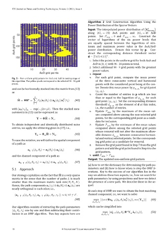
Fig. 5 – Non‐uniform grid pattern for AoA and AoD in testing stage of
the algorithm. The yellow pixels correspond to the selected 96 ⋅ 32 grid of the three consecutive vertical and horizontal
points. points with the considered point being at the cen‐
ter. Denote this mean power by for grid point
and can be horizontally stacked into the matrix from (13) ,
( , ).

as
5: Count the number of entries in p which are less
than or equal to the logarithm of for each
̂
,

= H = ∑ ̃ ( ̄ a ( ) ⊗ a ( )) ( ) (43) grid point ( , ). Set the corresponding distance
v
ℓ
ℓ
ℓ
ℓ
T
R

F

ℓ=1 threshold as the element of d at this index,
,
with [ ( )] = exp(− 2 ). Then the stacked mea‐ i.e., the number of entries.
F ℓ ℓ
6: Update by the maximum of the mean val‐
surements in (13) can be expressed as max
ues computed above among the non‐selected grid
̂
= + . (44) points. Set the corresponding grid point as a candi‐

date for inclusion.
To obtain independent and identically distributed noise 7: Update by the minimum of the mean values
min
entries, we apply the whitening given in (17), i.e., computed above among the selected grid points
whose removal will not alter the maximum allow‐
̂
Y = + N . (45)
w w w able distance between consecutive horizon‐
,
tal and vertical selected points. Set the correspond‐
To ease the notation, we will de ine the spatial component
ing grid point as a candidate for removal.
of a path as
8: Remove the grid point found in Step 7 from the grid
R−T ( , ) = ̄ a ( ) ⊗ a ( ) (46) pattern and add the grid point found in Step 6 to the
ℓ
ℓ
ℓ
ℓ
T
R
grid pattern.
9: until >
and the channel component of a path as min max
Output: The updated non‐uniform grid pattern
( , , ) = ( ) ⊗ ( , ). (47)
R−T−F ℓ ℓ ℓ F ℓ R−T ℓ ℓ
(a) how to set the dictionary for determining the path pa‐
rameters and (b) how to know when to stop the OMP it‐
5.1 Approach
erations. Key to the success of our algorithm lies in the
̂
Our strategy capitalizes on the fact that is a very sparse way we address these two aspects, i.e., how we search for
matrix in the sense that the number of paths is much path parameters by using projections and how we detect
smaller than the maximum matrix rank min( , ). the presence of a new path. We describe these in the se‐
t
r
Hence, the path components ( ) ⊗ ̄ a ( ) ⊗ a ( ) are quel.
ℓ
ℓ
ℓ
T
R
F
nearly orthogonal to each other, i.e.,
At each step of OMP, we want to obtain the best matching
′
⟨ ( , , ), ( ′, ′, ′)⟩ ≈ 0, ∀ℓ ≠ ℓ . channel component, i.e., we want to solve
R−T−F ℓ ℓ ℓ R−T−F ℓ ℓ ℓ
(48) max ∣⟨ ( ( , ) ( )), ( )⟩∣ (49)

R−T ℓ ℓ F ℓ w
ℓ , ℓ , ℓ
Our algorithm consists of extracting the path parameters which can be simpli ied into
( , , ) one by one and then subtracting their contri‐ max | ∗ ( , ) ( ))|, (50)
∗
ℓ
ℓ
ℓ
̄
bution in an OMP algorithm. Two key aspects here are ℓ , ℓ , ℓ R−T ℓ ℓ w F ℓ
18 © International Telecommunication Union, 2021