Page 29 - ITU Journal Future and evolving technologies Volume 2 (2021), Issue 4 – AI and machine learning solutions in 5G and future networks

ITU Journal on Future and Evolving Technologies, Volume 2 (2021), Issue 4

3.2 Multi‐level greedy search ̃
Input: Y , , ,
w w
, , Δ , Δ
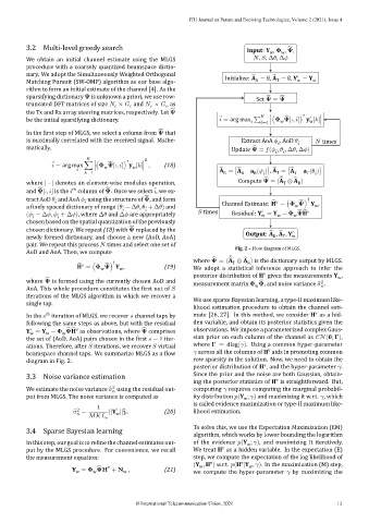
We obtain an initial channel estimate using the MLGS
procedure with a coarsely quantized beamspace dictio‐
nary. We adopt the Simultaneously Weighted Orthogonal Initialize: A = ∅, A = ∅, Y = Y
̂
̂
′
Matching Pursuit (SW‐OMP) algorithm as our base algo‐ R T w w
rithm to form an initial estimate of the channel [4]. As the
sparsifying dictionary is unknown a priori, we use row‐ Set =
̂
̃
truncated DFT matrices of size × and × as

̃
the Tx and Rx array steering matrices, respectively. Let ∗
̂
̂
′
be the initial sparsifying dictionary. = arg max ∑ =1 ∣( [∶, ]) y [ ]∣

w
w
̃
In the irst step of MLGS, we select a column from that
is maximally correlated with the received signal. Mathe‐ Extract AoA ̂ , AoD ̂ times
matically, ̂ , Δ , Δ )
Update = ( ̂ , ̂
∗ 2
̃
̂
= arg max ∑ ∣( [∶, ]) y [ ]∣ , (18)
̂
A = [ ̂
A
w w ̂ A )], A = [ ̂ )]
=1 R R a ( ̂ T T a ( ̂
T
R
̄
̂
̂
̂
Compute = (A ⊗ A )
where | ⋅ | denotes an element‐wise modulus operation, T R
̃
̃
̂
and [∶, ] is the column of . Once we select , we ex‐
th
̃
using the structure of , and form †
tract AoD ̂ and AoA ̂ ̂
̂ v
Channel Estimate: H = ( ) Y ,
w
w
a inely spaced dictionary of range ( ̂ − Δ , ̂ + Δ ) and
′
times Residual: Y = Y − H
̂̂ v
( ̂ − Δ , ̂ + Δ ), where Δ and Δ are appropriately w w w
chosen based on the spatial quantization of the previously
̃
chosen dictionary. We repeat (18) with replaced by the Output: A , A , Y ′
̂ ̂
newly formed dictionary, and choose a new {AoD, AoA} R T w
pair. We repeat this process times and select one set of
Fig. 2 – Flow diagram of MLGS.
AoD and AoA. Then, we compute
̂ ̂ ̄ ̂
† where = (A ⊗ A ) is the dictionary output by MLGS.
T
R
̂
H = ( ) Y , (19)
̂ v
w w We adopt a statistical inference approach to infer the
v
posterior distribution of H given the measurements Y ,
̂ w
̂
where is formed using the currently chosen AoD and measurement matrix , and noise variance ̂ .
2
AoA. This whole procedure constitutes the irst out of w
iterations of the MLGS algorithm in which we recover a
We use sparse Bayesian learning, a type‐II maximum like‐
single tap.
lihood estimation procedure to obtain the channel esti‐
v
th
In the iteration of MLGS, we recover channel taps by mate [26, 27]. In this method, we consider H as a hid‐
following the same steps as above, but with the residual den variable, and obtain its posterior statistics given the
′ ̂̂ v ̂ observations. We impose a parameterized complex Gaus‐
Y = Y − H as observations, where comprises
w w w
the set of {AoD, AoA} pairs chosen in the irst − 1 iter‐ sian prior on each column of the channel as (0, ),
where = diag( ). Using a common hyper‐parameter
ations. Therefore, after iterations, we recover virtual
v
across all the columns of H aids in promoting common
beamspace channel taps. We summarize MLGS as a low
diagram in Fig. 2. row sparsity in the solution. Now, we need to obtain the
v
posterior distribution of H , and the hyper‐parameter .
Since the prior and the noise are both Gaussian, obtain‐
3.3 Noise variance estimation
v
ing the posterior statistics of H is straightforward. But,
2
We estimate the noise variance ̂ using the residual out‐ computing requires computing the marginal probabil‐

put from MLGS. The noise variance is computed as ity distribution (Y ; ) and maximizing it w.r.t. , which
w
is called evidence maximization or type‐II maximum like‐
1
′
2
2 ̂ = ||Y || . (20) lihood estimation.
w

To solve this, we use the Expectation Maximization (EM)
3.4 Sparse Bayesian learning
algorithm, which works by lower bounding the logarithm
In this step, our goal is to re ine the channel estimates out‐ of the evidence (Y ; ), and maximizing it iteratively.
w
v
put by the MLGS procedure. For convenience, we recall We treat H as a hidden variable. In the expectation (E)
the measurement equation: step, we compute the expectation of the log likelihood of
v
v
(Y , H ) w.r.t. (H |Y , ). In the maximization (M) step,
w
w
̂
v
Y = H + N , (21) we compute the hyper‐parameter by maximizing the
w
w
w
© International Telecommunication Union, 2021 13