Page 33 - ITU Journal Future and evolving technologies Volume 2 (2021), Issue 4 – AI and machine learning solutions in 5G and future networks

ITU Journal on Future and Evolving Technologies, Volume 2 (2021), Issue 4

⎛ | | ⎞
⎟
⎜
( +1) = Π ⎜ 2 ⎟ (37)
⎟
⎜
⎜
⎟
∑ (∥y − A ( ) ∥ + ( ( ) ) −1 ( − tr ( ( ) D )))

( )
⎝ ∈ ⎠
6
10
y = x + n . (40) 16
training training training
14
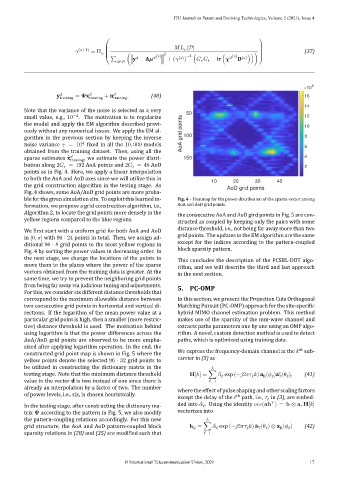
Note that the variance of the noise is selected as a very 50
−4 12
small value, e.g., 10 . The motivation is to regularize
the model and apply the EM algorithm described previ‐ 10
ously without any numerical issues. We apply the EM al‐ AoA grid points
gorithm in the previous section by keeping the inverse 100 8
4
noise variance = 10 ixed in all the 10, 000 models 6
obtained from the training dataset. Then, using all the
sparse estimates ̂ x , we estimate the power distri‐ 150 4
training
bution along 2 = 192 AoA points and 2 = 48 AoD 2

points as in Fig. 4. Here, we apply a linear interpolation
to both the AoA and AoD axes since we will utilize this in
10 20 30 40
the grid construction algorithm in the testing stage. As AoD grid points
Fig. 4 shows, some AoA/AoD grid points are more proba‐
ble for the given simulation site. To exploit this learned in‐ Fig. 4 – Heatmap for the power distribution of the sparse vector among
formation, we propose a grid construction algorithm, i.e., AoA and AoD grid points.
Algorithm 2, to locate the grid points more densely in the the consecutive AoA and AoD gird points in Fig. 5 are con‐
yellow regions compared to the blue regions.
structed as coupled by keeping only the pairs with some
distance threshold, i.e., not being far away more than two
We irst start with a uniform grid for both AoA and AoD
in [0, ] with 96 ⋅ 24 points in total. Then, we assign ad‐ grid points. The updates in the EM algorithm are the same
except for the indices according to the pattern‐coupled
ditional 96 ⋅ 8 grid points to the most yellow regions in
block sparsity pattern.
Fig. 4 by sorting the power values in decreasing order. In
the next stage, we change the locations of the points to This concludes the description of the PCSBL‐DDT algo‐
move them to the places where the power of the sparse
rithm, and we will describe the third and last approach
vectors obtained from the training data is greater. At the
in the next section.
same time, we try to prevent the neighboring grid points
5. PC‑OMP
from being far away via judicious tuning and adjustments.
For this, we consider six different distance thresholds that
correspond to the maximum allowable distance between In this section, we present the Projection Cuts Orthogonal
two consecutive grid points in horizontal and vertical di‐ Matching Pursuit (PC‐OMP) approach for the site‐speci ic
rections. If the logarithm of the mean power value at a hybrid MIMO channel estimation problem. This method
particular grid point is high, then a smaller (more restric‐ makes use of the sparsity of the mm‐wave channel and
tive) distance threshold is used. The motivation behind extracts paths parameters one by one using an OMP algo‐
using logarithm is that the power differences across the rithm. A novel, custom detection method is used to detect
AoA/AoD grid points are observed to be more empha‐ paths, which is optimized using training data.
sized after applying logarithm operation. In the end, the
th
We express the frequency‐domain channel at the sub‐
constructed grid point map is shown in Fig. 5 where the
carrier in (5) as
yellow points denote the selected 96 ⋅ 32 grid points to
be utilized in constructing the dictionary matrix in the
∗
testing stage. Note that the minimum distance threshold [ ] = ∑ ̃ exp (− 2 ) a ( )a ( ), (41)
ℓ
ℓ
ℓ
ℓ
R
T
value in the vector d is two instead of one since there is ℓ=1
already an interpolation by a factor of two. The number
where the effect of pulse shaping and other scaling factors
of power levels, i.e., six, is chosen heuristically. th
except the delay of the ℓ path, i.e., in (3), are embed‐
ℓ

In the testing stage, after constructing the dictionary ma‐ ded into ̃ . Using the identity ( ) = ⊗ , [ ]
ℓ
trix according to the pattern in Fig. 5, we also modify vectorizes into
the pattern‐coupling relations accordingly. For this new
grid structure, the AoA and AoD pattern‐coupled block = ∑ ̃ exp (− 2 ) ̄ a ( ) ⊗ a ( ) (42)
ℓ
ℓ

ℓ
ℓ
T
R
sparsity relations in (28) and (35) are modi ied such that ℓ=1
© International Telecommunication Union, 2021 17