Page 30 - ITU Journal Future and evolving technologies Volume 2 (2021), Issue 4 – AI and machine learning solutions in 5G and future networks

ITU Journal on Future and Evolving Technologies, Volume 2 (2021), Issue 4

̂
Input: Y , , , ̂ domain sparsity to denoise the channel to further reduce
w w
the MSE between the original and estimated channels.
̄
̂
̂
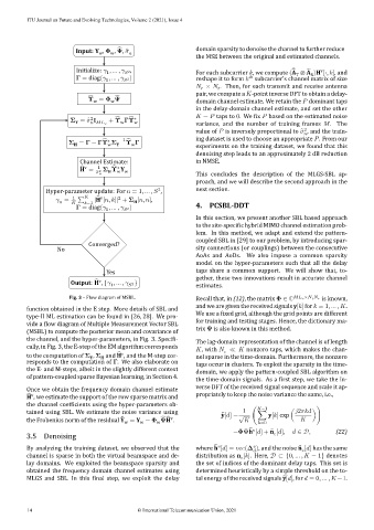
Initialize: , … , , For each subcarrier , we compute (A ⊗ A )H [∶, ], and
2
v
1

R

= diag( , … , ) reshape it to form subcarrier’s channel matrix of size

2
1

× for tr receiv antenna

pair, we compute a ‐point inverse DFT to obtain a delay‐
̂
̂
= domain channel estimate. We retain the dominant taps
w
w
in the delay‐domain channel estimate, and set the other
̂
= ̂ I + w − taps to 0 We ix based on the estimated noise
̂ ∗
2
Y
v of tr fr
w

The
2
value of is inversely proportional to ̂ , and the train‐

̂
̂ ∗
= − −1 ing dataset is used to choose an appropriate . From our
H
Y
w
w
experiments training dataset we found that this
denoising step leads to an approximately 2 dB reduction
Channel Estimate: in NMSE.
̂ ∗
H = 1 2 Y
̂ v
H
̂ w w This description of MLGS‐ ap‐
proach, and we will describe the second approach in the
2 next section.
Hyper‐parameter update: For = 1, … , ,
2
1
= ∑ |H [ , ]| + [ , ],
̂ v
H

=1
= diag( , … , ) 4. PCSBL‑DDT
1
2

In this section, we present another SBL based approach
to the site‐speci ic hybrid MIMO channel estimation prob‐
w adapt ext pattern‐
coupled SBL in [29] to our problem, by introducing spar‐
Converged?
No sity connections (or couplings) between the consecutive
A AoDs. W impose sparsity
hyper‐parameters that all delay
taps shar support W will sho that to‐
Yes
gether, these two innovations result in accurate channel
Output: H , { , … , } estimates.
̂ v
2

1
Fig. 3 – Flow diagram of MSBL. Recall that, in (12), the matrix ∈ ℂ × is known,
and we are given the received signals y[ ] for = 1, … , .
function obtained in the E st More details of SBL and
type‐II ML estimation can be found in [26, 28 We pro‐ We use a ixed grid, although the grid points are different
for training and testing stages. Hence, the dictionary ma‐
vide a low diagram of Multiple Measurement Vector SBL
trix is also known in this method.
(MSBL) to compute the posterior mean and covariance of
the channel, and the hyper‐parameters, in 3 Speci i‐
The lag‐domain representation of the channel is of length
cally, in Fig. 3, the E‐step of the EM algorithm corresponds
, with ≪ nonzero taps, which makes the chan‐

̂ v
to the computation of , and H , and the M‐step cor‐ nel sparse in the time‐domain. Furthermore, the nonzero
Y
H
responds to the computation of We also elaborate on taps occur in clusters. To exploit the sparsity in the time‐
the E‐ and M‐steps, albeit in the slightly different context
domain, we apply the pattern‐coupled SBL algorithm on
of pattern‐coupled sparse Bayesian learning, in Section 4.
the time‐domain As a irst step, we take the in‐
verse DFT of the received signal sequence and scale it ap‐
Once we obtain the frequency domain channel estimate
̂ v propriately to keep the noise variance the same, i.e.,
H , we estimate the support of the row sparse matrix and
the channel coef icients using the hyper‐parameters ob‐ −1
W estimat noise v using ̃ y[ ] =√ 1 (∑ y[ ] exp ( 2 ))
̃
the Frobenius of residual Y = Y − ̂̂ v
H .
e
w =0
̃
= h [ ] + ̃ n [ ], ∈ , (22)

Denoising
̃
analyzing dataset, observed that the where h [ ] = ( ), and the noise ̃ n [ ] has the same

channel is sparse in both the virtual beamspace and de‐ distribution as n [ ]. Here, ⊂ {0, … , − 1} denotes

lay domains. sparsity and the set of indices of the dominant delay taps. This set is
obtained the frequency domain channel estimates using determined heuristically by a simple threshold on the to‐
MLGS and SBL. In this inal step, we exploit the delay tal energy of the received signals ̃ y[ ], for = 0, … , −1.
14 © International Telecommunication Union, 2021