Page 89 - Kaleidoscope Academic Conference Proceedings 2024

Innovation and Digital Transformation for a Sustainable World

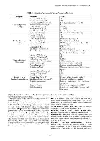
Table 3 – Simulation Parameters for Various Approaches Proposed

Category Parameter Value
Number of Vehicles ( ) 10
Number of Time Steps ( ) 100
Total Spectrum Over Time ( ) Linearly increases from 10 to 100
Dynamic Spectrum Regularization Parameter ( ) 0.1

Sharing Utility Function ( , ( )) sin 2 ·

Penalty Function ( ( )) · var( )
Initial Spectrum Allocation Based on historical data
Optimization Strategy Minimize total utility and penalty
Number of Vehicles 10
Number of Time Steps 100
Traffic Data Distribution Normal(loc=50, scale=10)
Machine Learning Resource Usage Pattern Normal(loc=0.5, scale=0.1)
Models Neural Network Architecture MLPRegressor, hidden layers=100,
max_iter=500
Learning Rate (RL) 0.01
Initial Policy Parameter (Θ) Random initialization
Reward Function Negative of absolute difference between
predicted and actual resource usage
Number of Vehicles ( ) 10
Number of Time Steps ( ) 50
Trade-off Parameters ( , ) 0.8, 0.2
Adaptive Resource
Maximum Total Resources ( ) 100 for each vehicle
Management
Utility Function ( , ) Random values between 0 and 1
Penalty Function ( , ) Random values between 0 and 1
Optimization Model Maximize weighted sum of utility minus
penalty
Number of Users/Vehicles ( ) 10
Number of Time Steps ( ) 100
2
Noise Power ( ) 0.1
Beamforming in Channel State Matrix (H) Complex values, generated randomly
Sidelink Communication Initial Beamforming Vectors (W) Randomly initialized, normalized
Optimization Approach Iterative adjustment to maximize
throughput
Objective Function Maximize sum log function of SINR
SINR Calculation Based on beamforming vectors and
interference

Figure 2 presents a heatmap of the dynamic spectrum 5.2 Machine Learning Models
allocation among vehicles over time.
Y-axis (Vehicle): Lists the vehicles involved in sidelink V2X Figure 3 shows the predictive resource allocation for a
communication. single vehicle using a neural network model. The blue line
X-axis (Time): Indicates the time progression. represents actual resource usage, while the dashed orange line
Color Intensity: Shows the spectrum amount allocated shows predicted usage over time.
to each vehicle, with brighter colors indicating higher Actual Resource Usage (Blue Line): The true resource
allocations. Interpretation: The heatmap reveals allocation consumption of the vehicle across time steps.
patterns, showing how the system adapts to changing vehicle Predicted Resource Usage (Dashed Orange Line):
demands and conditions. It highlights vehicles consistently Resource usage predicted by the neural network model.
receiving more spectrum due to utility and proximity Interpretation: The close alignment between actual and
considerations. Relevance to 6G V2X Standardization: predicted values demonstrates the model’s effectiveness in
The dynamic spectrum allocation strategies demonstrated forecasting resource needs, optimizing network efficiency by
here illustrate how future 6G systems can efficiently anticipating demand.
manage spectrum resources in real-time, ensuring both high Relevance to 6G V2X Standardization: Predictive
performance and fairness. models ensure resources are allocated based on future
needs, minimizing wastage and improving overall network
performance. The model can be retrained periodically

– 45 –