Page 418 - Kaleidoscope Academic Conference Proceedings 2024

2024 ITU Kaleidoscope Academic Conference

1) User Latency v/s UAV – Altitude: Fig. 2 shows the 3) Optimization function v/s UAV-Altitude (for different
trend of user latency with respect to the UAV altitude, where PL max values): The optimization function here is considered
the UAV altitude is varied between the 0 to 3200 meters with λ value of 0.5, i.e. taking λ = 0.5 in eq.(21). Thus, the
(The maximum possible altitude for a UAV with cell user minimum altitude for optimization function is optimizing the
path−loss < 110 dB). The user latency accounts for both power and latency functions in equal proportions, as shown in
the transmission delay and the propagation delay, if a UDP Fig. 4. The curve also shows the variations of the optimization
data packet is to be transmitted from UAV to a ground based function curve for different PL max values. As the PL max
UE. It can be observed that the user latency follows a bell is increased, the maximum attainable altitude of the UAV
shaped curve. The propagation delay for low range UAV also increases. The optimization point also shifts slightly to
(< 1.5km) is negligible compared to the transmission delay. a higher UAV elevation as the PL max is increased.
Thus, the latency is dominated by transmission delay or more
appropriately the bitrate.

Fig. 5. Optimization Function vs UAV Altitude (for different densities)

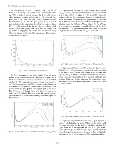
4) Optimization function v/s UAV-Altitude (for different user
densities): λ = 0.5 is considered here, to observe the variation
Fig. 3. Power Consumption vs UAV Altitude
in the optimization function with varying UAV altitudes, and
2) Power Consumption v/s UAV-Altitude: From the power depicted in Fig. 5, which is plotted for different user densities.
model, it can be seen that power consumed is proportional to Three cases are considered (i.e. low, medium and high user
the UAV swarm size. The UAV swarm size is the minimum density). As the user density increases, the optimization curve
number of UAVs required to provide coverage to a given area shifts in the y direction and the optimum elevation also shifts
A T . The coverage area of a UAV changes with its altitude and to a lower value.
is maximum at the optimum altitude where the coverage radius
is maximum [5]. Thus power consumption plot, as shown in
Fig. 3, forms a U shaped curve with the minimum at the
optimum UAV altitude. However, since the swarm size is a
discrete number, a step variation in the power latency plot can
be observed.

Fig. 6. Optimization Function vs UAV Altitude (for different λ values)

5) Optimization function v/s UAV-Altitude (for different λ
values): λ is balancing the trade-off between the latency and
the power functions in the final optimization function. For
higher value of λ, the optimum altitude is a higher value,
as the optimum points shifts towards right (towards optimum
Fig. 4. Optimization Function vs UAV Altitude (for different PL max values) point of the power function), as depicted in Fig. 6. Similarly
for lower values of λ, the optimum UAV elevation reduces.

– 374 –