Page 52 - ITU Journal, Future and evolving technologies - Volume 1 (2020), Issue 1, Inaugural issue

ITU Journal on Future and Evolving Technologies, Volume 1 (2020), Issue 1

4 3
4
2
2
1.5
2
Amplitude 1 0 1
2
0.5 0 0
0 -2 -2 -1
0 500 1000 1500 2000 2500 3000 3500 4000 0 200 400 600 800 1000 1200 1400 1600 1800 2000 0 200 400 600 800 1000 1200 1400 1600 1800 2000 0 200 400 600 800 1000 1200 1400 1600 1800 2000
Original Signal Approximation Approximation Approximation
4 1 2 1 2 1
Amplitude 2 0.5 0 0 0
0
-0.5 -1 -1
-2 -1 -2 -2
0 500 1000 1500 2000 2500 3000 3500 4000 0 200 400 600 800 1000 1200 1400 1600 1800 2000 0 200 400 600 800 1000 1200 1400 1600 1800 2000 0 200 400 600 800 1000 1200 1400 1600 1800 2000
Noisy Signal Detail Detail Detail
(a) (b) (c) (d)
3 4 3 3
2 2
2 2
1 1
0 1
0 0
-1 -2 -1 0
0 200 400 600 800 1000 1200 1400 1600 1800 2000 0 200 400 600 800 1000 1200 1400 1600 1800 2000 0 200 400 600 800 1000 1200 1400 1600 1800 2000 0 200 400 600 800 1000 1200 1400 1600 1800 2000
Approximation Approximation Approximation Approximation
2 2 2 2
1 1 1 1
0 0 0 0
-1 -1 -1 -1
-2 -2 -2 -2
0 200 400 600 800 1000 1200 1400 1600 1800 2000 0 200 400 600 800 1000 1200 1400 1600 1800 2000 0 200 400 600 800 1000 1200 1400 1600 1800 2000 0 200 400 600 800 1000 1200 1400 1600 1800 2000
Detail Detail Detail Detail
(e) (f) (g) (h)
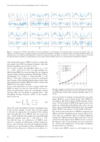
Fig. 9 – Comparison of MSICA with different wavelet transforms in decomposing a PieceRegular signal corrupted by impulse noise. (a)
Original and Noisy Signal; (b) Approximation and detail by Daubechies 3 wavelet; (c) Approximation and detail by Haar wavelet; (d)
Approximation and detail by Biorthogonal 2.2 wavelet; (e) Approximation and detail by Coiflets 4 wavelet; (f) Approximation and detail
by Fejer-Korovkin 4 wavelet; (g) Approximation and detail by discrete Meyer wavelet; (h) Approximation and detail by MSICA.
cally independent; hence, MSICA is able to extract the
noise signal from CH2 (via channel diversity), while the 0.14
wavelet transforms are not able to do so. 0.12 Daubechies 3
Fig. 8 shows a signal decomposition where 2 = 0.2, 0.1 Haar
Biorthogonal 2.2
= 0.05. As it can be seen, the approximation ob- Coiflets 4
Fejer-Korovkin 4
1
tained using MSICA is less noisy than the one obtained 0.08 MSICA
using the other wavelet transforms (Daubechies 3, Haar, MSE 0.06
Biorthogonal 2.2, Coiflets 4, Fejer-Korovkin 4, and
Meyer). This result confirms our statement and shows 0.04
that, because of the statistical independenc between the 0.02
approximation and detail, MSICA is able to extract the
AWGN from the noisier channel. 0 0.2 0.4 0.6 0.8 1 1.2 1.4 1.6 1.8 2
In the other experiment, in order to show visibly that P a ×10 -3
MSICA is able to extract the noise of CH2, we have ex- Fig. 10 – Impulse noise rejection in terms of Minimum Square Er-
plored its performance when the odd samples, passed ror (MSE); MSICA performance does not depend on , whereas
through CH2, are corrupted by impulse noise. The the performance of the other transforms decreases when in-
Probability Density Function (PDF) of the impulse creases.
noise is given as, tract accurately the impulse components from the noisy
signal. However, as it is shown in Fig. 9(h), MSICA is
⎧ = , successful as the detail contains all the impulse compo-
{
( ) = = − , (36)
⎨ = 0, nents. This is because in MSICA the approximation and
{
⎩ 1 − 2
detail are statistically independent and, since the im-
where 2 is the probability of existence of impulse noise pulse noise is statistically independent from the original

in the received samples. In Fig. 9(a), the noisy signal signal, MSICA can extract it in the detail coefficients.
is obtained by passing the even samples of the original Fig. 10 shows the performance of MSICA compared with
signal through CH1 with AWGN with zero mean and different wavelet transforms when various values of ,

2 = 0.004, while the odd samples were passed through as in (36), are considered. Here, the detail coefficients
2 obtained by different methods have been set to zero to
CH2 with impulse noise ( = 0.01 and = 1.5).
Fig. 9(b)-(h) show the performance of MSICA com- denoise the noisy signal. Since MSICA is able to extract
pared to a number of well-known wavelet transforms. the impulse noise, its performance does not depend on
As it is clear from Fig. 9(b)-(g), the traditional wavelet , whereas the performance of the other transforms

transforms (i.e., Daubechies 3, Haar, Biorthogonal 2.2, decreases when increases.

Coiflets 4, Fejer-Korovkin 4, Meyer) are not able to ex- To show that MSICA works on real signals too, we

32 © International Telecommunication Union, 2020