Page 50 - ITU Journal, Future and evolving technologies - Volume 1 (2020), Issue 1, Inaugural issue

ITU Journal on Future and Evolving Technologies, Volume 1 (2020), Issue 1

or space [30]) and 2) denoising in the transform domain
(e.g., using Fourier or a wavelet transform [31, 32]). 0.07
Since the wavelet transform provides information in
both the time and frequency domain, and the infor- 0.06 Daubechies 3
Haar
mation in one scale is not contained in another scale, 0.05 Biorthogonal 2.2
approaches in this second category can strike a balance Coiflets 4
Fejer-Korovkin 4
between noise suppression and signal structural preser- 0.04 MSICA
vation, and have therefore been used widely in signal de- MSE
noising. It is interesting to note that, usually, the detail 0.03
coefficients of a noiseless signal are sparse. This means
that in the wavelet transform most of the detail coeffi- 0.02
cients of a noiseless signal are very small/close to zero
(as can be seen, for instance, in Fig. 4). So, the detail 0.01
coefficients with a small magnitude can be considered as
a noise component and can be set to zero. This is the 0 0.1 0.15 0.2 0.25 0.3 0.35 0.4 0.45 0.5
basic idea of wavelet thresholding approaches, which are w
employed in signal denoising where the coefficients are
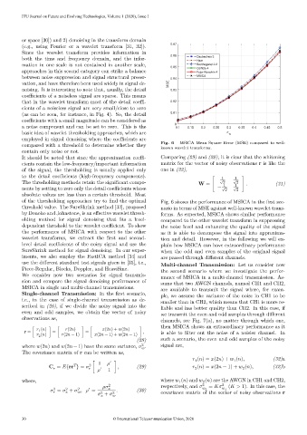
compared with a threshold to determine whether they Fig. 6 – MSICA Mean Square Error (MSE) compared to well-
known wavelet transforms.
contain only noise or not.
It should be noted that since the approximation coeffi- Comparing (29) and (20), it is clear that the whitening
cients contain the low-frequency/important information matrix for the vector of noisy observations r is like the
of the signal, the thresholding is usually applied only one in (22),
to the detail coefficients (high-frequency components). 1 1
The thresholding methods retain the significant compo- W = [ √ 2 √ 2 ] . (31)
nents by setting to zero only the detail coefficients whose − √ 1 2 √ 1 2
absolute values are less than a certain threshold. Most
of the thresholding approaches try to find the optimal Fig. 6 shows the performance of MSICA in the first sce-
threshold value. The SureShrink method [33], proposed nario in terms of MSE against well-known wavelet trans-
by Donoho and Johnstone, is an effective wavelet thresh- forms. As expected, MSICA shows similar performance
olding method for signal denoising that fits a level- compared to the other wavelet transform in suppressing
dependent threshold to the wavelet coefficient. To show the noise level and enhancing the quality of the signal
the performance of MSICA with respect to the other as it is able to decompose the signal into approxima-
wavelet transforms, we extract the first and second- tion and detail. However, in the following we will ex-
level detail coefficients of the noisy signal and use the plain how MSICA can have extraordinary performance
SureShrink method for signal denoising. In our exper- when the odd and even samples of the original signal
iments, we also employ the FastICA method [34] and are passed through different channels.
use the different standard test signals given in [35], i.e., Multi-channel Transmission: Let us consider now
Piece-Regular, Blocks, Doppler, and HeaviSine. the second scenario where we investigate the perfor-
We consider now two scenarios for signal transmis- mance of MSICA in a multi-channel transmission. As-
sion and compare the signal denoising performance of sume that two AWGN channels, named CH1 and CH2,
MSICA in single and multi-channel transmissions. are available to transmit the signal where, for exam-
Single-channel Transmission: In the first scenario, ple, we assume the variance of the noise in CH1 to be
i.e., in the case of single-channel transmission as de- smaller than in CH2, which means that CH1 is more re-
scribed in (26), if we divide the noisy signal into the liable and has better quality than CH2. In this case, if
even and odd samples, we obtain the vector of noisy we transmit the even and odd samples through different
observations as, channels, see Fig. 7(a), no matter through which one,
then MSICA shows an extraordinary performance as it
( ) (2 ) (2 ) + (2 )
r = [ 1 ] = [ ] = [ ] , is able to filter out the noise of a noisier channel. In
( ) (2 − 1) (2 − 1) + (2 − 1)
2
(28) such a scenario, the even and odd samples of the noisy
where (2 ) and (2 −1) have the same variance, . signal are,
2

The covariance matrix of r can be written as,
( ) = (2 ) + ( ), (32)a
1
1
1 ′
2

C = {rr } = [ ′ 1 ] , (29) ( ) = (2 − 1) + ( ), (32)b
2

2
where, where ( ) and ( ) are the AWGN in CH1 and CH2,
2
1
2 respectively, and 2 = 2 ( > 1). In this case, the

2
′
2
2
= + , = + 2 . (30) covariance matrix of the vector of noisy observations r
2
1

2

30 © International Telecommunication Union, 2020