
Page 49 - ITU Journal, Future and evolving technologies - Volume 1 (2020), Issue 1, Inaugural issue
P. 49
ITU Journal on Future and Evolving Technologies, Volume 1 (2020), Issue 1
2 3 3 3
1.8
2 2 2
1.6
1 1 1
1.4
1.2 0 0 0
Amplitude 0.8 1 0.4 0 200 400 600 800 Approximation 1400 1600 1800 2000 1 0 200 400 600 800 Approximation 1400 1600 1800 2000 0.4 0 200 400 600 800 Approximation 1400 1600 1800 2000
1200
1000
1200
1000
1000
1200
0.6 0.2 0.5 0.2
0.4 0 0 0
0.2 -0.2 -0.5 -0.2
0 -0.4 -1 -0.4
0 500 1000 1500 2000 2500 3000 3500 4000 0 200 400 600 800 1000 1200 1400 1600 1800 2000 0 200 400 600 800 1000 1200 1400 1600 1800 2000 0 200 400 600 800 1000 1200 1400 1600 1800 2000
Original Signal Detail Detail Detail
(a) (b) (c) (d)
3
3 3 3
2
2 2 2
1 1 1 1
0 0 0 0
0 200 400 600 800 1000 1200 1400 1600 1800 2000 0 200 400 600 800 1000 1200 1400 1600 1800 2000 0 200 400 600 800 1000 1200 1400 1600 1800 2000 0 200 400 600 800 1000 1200 1400 1600 1800 2000
Approximation Approximation Approximation Approximation
0.4
0.4 1 1
0.2
0.2 0.5 0.5
0 0 0 0
-0.2 -0.5 -0.2 -0.5
-0.4 -1 -0.4 -1
0 200 400 600 800 1000 1200 1400 1600 1800 2000 0 200 400 600 800 1000 1200 1400 1600 1800 2000 0 200 400 600 800 1000 1200 1400 1600 1800 2000 0 200 400 600 800 1000 1200 1400 1600 1800 2000
Detail Detail Detail Detail
(e) (f) (g) (h)
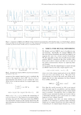
Fig. 4 – Comparison of MSICA with different wavelet transforms in decomposing a Piece-Regular signal. (a) Original Signal. Approxi-
mation and detail by (b) Daubechies 3 wavelet; (c) Haar wavelet; (d) Biorthogonal 2.2 wavelet; (e) Coiflets 4 wavelet; (f) Fejer-Korovkin
4 wavelet; (g) discrete Meyer wavelet; and (h) our proposed MSICA.
2 4. MSICA FOR SIGNAL DENOISING
1.8
We discuss now how MSICA can be beneficial in sig-
nal denoising. Specifically, we compare MSICA with
1.6
1.4 the other wavelet transforms and show how MSICA can
suppress the noise via a simple wavelet thresholding.
1.2
Amplitude 1 We also show that, in the case of multi-channel trans-
mission, MSICA outperforms the other wavelet trans-
forms and is able to extract and filter out the noise of
0.8
the noisier communication channel by exploiting chan-
0.6
nel diversity.
0.4
Let us assume that the original signal is passed through
0.2
an AWGN channel, the noisy output signal is then,
0
0 500 1000 1500 2000 2500 3000 3500 4000
Reconstructed Signal ( ) = ( ) + ( ) , = 1, … , , (26)
Fig. 5 – Reconstructed signal by MSICA using the approximation where ( ) is the original signal and ( ) is the AWGN
and detail in Fig. 4(h).
with zero mean and variance of . The goal of sig-
2
reconstruct the original signal we need to multiply the nal denoising is to remove the noise and obtain an es-
inverse of the separation matrix (B ) by the vector of timate ̂ ( ) of ( ) that minimizes the Mean Squared
−1
approximation and detail y so as to obtain the obser- Error (MSE), defined as,
vation vector x and reconstruct the original signal ( )
from x, i.e., 1 2
MSE ( ̂ ) = ∑ ( ̂ ( ) − ( )) . (27)
=1
( )
−1
[ 1 ] = x = B y, (24) Note that the model presented in (26) is not general
( )
since the noise may be non-additive, and the relation
2
between the noisy observed signal and the original signal
( ) = ( ( ) ↑ 2) + ( ( ) ↑ 2) ∗ ( + 1), (25) may be stochastic. Nevertheless, (26) is a widely used
2
1
model in many practical situations as it serves well as
where ( ) ↑ 2, = 1, 2, denotes the upsampling of a motivating example to give a good sense as to what
( ) by a factor of 2. Fig. 5 shows the reconstructed sig- happens in more realistic channels.
nal using (24) and (25). This figure shows that MSICA Let us emphasize that there are many existing ap-
can successfully reconstruct the original signal from the proaches in the literature to perform signal denoising,
approximation and detail obtained in the decomposition which can be roughly divided into two main categories:
procedure. 1) denoising in the original signal domain (e.g., in time
© International Telecommunication Union, 2020 29