Page 51 - ITU Journal, Future and evolving technologies - Volume 1 (2020), Issue 1, Inaugural issue

ITU Journal on Future and Evolving Technologies, Volume 1 (2020), Issue 1

0.04 14
13
0.035
Daubechies 3 Daubechies 3
Haar 12 Haar
0.03 Biorthogonal 2.2 Biorthogonal 2.2
Coiflets 4 11 Coiflets 4
0.025 Fejer-Korovkin 4 Fejer-Korovkin 4
MSICA 10 MSICA
MSE 0.02 SNRI 9
8
0.015
7
0.01
6
0.005
5
0 4
1 1.5 2 2.5 3 3.5 4 4.5 5 1 1.5 2 2.5 3 3.5 4 4.5 5
/ /
w 2 w 1 w 2 w 1
(a) (b) (c)
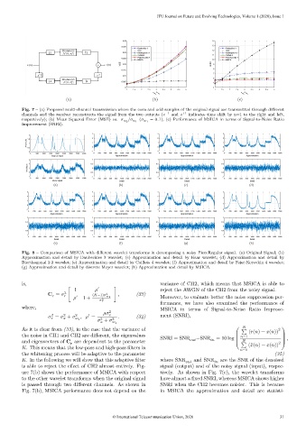
Fig. 7 – (a) Proposed multi-channel transmission where the even and odd samples of the original signal are transmitted through different
channels and the receiver reconstructs the signal from the two outputs ( −1 and +1 indicates time shift by n=1 to the right and left,
= 0.1); (c) Performance of MSICA in terms of Signal-to-Noise Ratio
respectively); (b) Mean Squared Error (MSE) vs. 2 / 1 ( 1
Improvement (SNRI).
3 3 3
2
2 2 2
1.5
Amplitude 1 1 1 1
0.5 0 0 0
0 -1 -1 -1
0 500 1000 1500 2000 2500 3000 3500 4000 0 200 400 600 800 1000 1200 1400 1600 1800 2000 0 200 400 600 800 1000 1200 1400 1600 1800 2000 0 200 400 600 800 1000 1200 1400 1600 1800 2000
Original Signal Approximation Approximation Approximation
3 1 1 1
Amplitude 2 1 0.5 0 0.5 0 0.5 0
-1 0 -0.5 -1 -0.5 -1 -0.5 -1
0 500 1000 1500 2000 2500 3000 3500 4000 0 200 400 600 800 1000 1200 1400 1600 1800 2000 0 200 400 600 800 1000 1200 1400 1600 1800 2000 0 200 400 600 800 1000 1200 1400 1600 1800 2000
Noisy Signal Detail Detail Detail
(a) (b) (c) (d)
3 3 3 3
2 2 2
2
1 1 1
1
0 0 0
-1 -1 -1 0
0 200 400 600 800 1000 1200 1400 1600 1800 2000 0 200 400 600 800 1000 1200 1400 1600 1800 2000 0 200 400 600 800 1000 1200 1400 1600 1800 2000 0 200 400 600 800 1000 1200 1400 1600 1800 2000
Approximation Approximation Approximation Approximation
1 1 1 1
0.5 0.5 0.5 0.5
0 0 0 0
-0.5 -0.5 -0.5 -0.5
-1 -1 -1 -1
0 200 400 600 800 1000 1200 1400 1600 1800 2000 0 200 400 600 800 1000 1200 1400 1600 1800 2000 0 200 400 600 800 1000 1200 1400 1600 1800 2000 0 200 400 600 800 1000 1200 1400 1600 1800 2000
Detail Detail Detail Detail
(e) (f) (g) (h)
Fig. 8 – Comparison of MSICA with different wavelet transforms in decomposing a noisy PieceRegular signal. (a) Original Signal; (b)
Approximation and detail by Daubechies 3 wavelet; (c) Approximation and detail by Haar wavelet; (d) Approximation and detail by
Biorthogonal 2.2 wavelet; (e) Approximation and detail by Coiflets 4 wavelet; (f) Approximation and detail by Fejer-Korovkin 4 wavelet;
(g) Approximation and detail by discrete Meyer wavelet; (h) Approximation and detail by MSICA.
is, variance of CH2, which means that MSICA is able to
1 ′ reject the AWGN of the CH2 from the noisy signal.
2
C = [ 2 ] , (33)

′ 1 + ( −1) 1 Moreover, to evaluate better the noise suppression per-
2
formance, we have also examined the performance of
where, MSICA in terms of Signal-to-Noise Ratio Improve-
2

2
′
2
= + 2 1 , = + 2 . (34) ment (SNRI),

2

1
As it is clear from (33), in the case that the variance of ∑ ( ( ) − ( )) 2

⎛
the noise in CH1 and CH2 are different, the eigenvalues SNRI = SNR −SNR = 10 log ⎜ ⎞
⎟
⎜ =1
⎟ ,
and eigenvectors of C are dependent to the parameter ⎜ 2 ⎟
⎜
⎟
r
∑ ( ̂ ( ) − ( ))
. This means that the low-pass and high-pass filters in ⎝ =1 ⎠
the whitening process will be adaptive to the parameter (35)
. In the following we will show that this adaptive filter where SNR and SNR are the SNR of the denoised
is able to reject the effect of CH2 almost entirely. Fig- signal (output) and of the noisy signal (input), respec-
ure 7(b) shows the performance of MSICA with respect tively. As shown in Fig. 7(c), the wavelet transforms
to the other wavelet transforms when the original signal have almost a fixed SNRI, whereas MSICA shows higher
is passed through two different channels. As shown in SNRI when the CH2 becomes noisier. This is because
Fig. 7(b), MSICA performance does not depend on the in MSICA the approximation and detail are statisti-
© International Telecommunication Union, 2020 31