
Page 47 - ITU Journal, Future and evolving technologies - Volume 1 (2020), Issue 1, Inaugural issue
P. 47
ITU Journal on Future and Evolving Technologies, Volume 1 (2020), Issue 1
0.5
0.5 1.5 0.8
s 2 0 x 2 0 z 2 0 y 2 0
-0.5 -1.5 -0.8 -0.5
-0.5 0 0.5 -1.5 0 1.5 -2.5 0 2.5 -1 0 1
s 1 x 1 z 1 y 1
(a) (b) (c) (d)
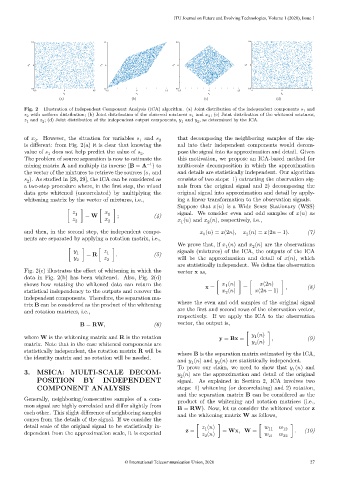
Fig. 2 – Illustration of Independent Component Analysis (ICA) algorithm. (a) Joint distribution of the independent components 1 and
2 with uniform distribution; (b) Joint distribution of the observed mixtures 1 and 2 ; (c) Joint distribution of the whitened mixtures,
1 and 2 ; (d) Joint distribution of the independent output components, 1 and 2 , as determined by the ICA.
of . However, the situation for variables and 2 that decomposing the neighboring samples of the sig-
1
2
is different: from Fig. 2(a) it is clear that knowing the nal into their independent components would decom-
value of does not help predict the value of . pose the signal into its approximation and detail. Given
1
2
The problem of source separation is now to estimate the this motivation, we propose an ICA-based method for
mixing matrix A and multiply its inverse (B = A ) to multi-scale decomposition in which the approximation
−1
the vector of the mixtures to retrieve the sources ( and and details are statistically independent. Our algorithm
1
). As studied in [28, 29], the ICA can be considered as consists of two steps: 1) extracting the observation sig-
2
a two-step procedure where, in the first step, the mixed nals from the original signal and 2) decomposing the
data gets whitened (uncorrelated) by multiplying the original signal into approximation and detail by apply-
whitening matrix by the vector of mixtures, i.e., ing a linear transformation to the observation signals.
Suppose that ( ) is a Wide Sense Stationary (WSS)
signal. We consider even and odd samples of ( ) as
[ 1 ] = W [ 1 ] ; (4)
2 2 ( ) and ( ), respectively, i.e.,
1
2
and then, in the second step, the independent compo- ( ) = (2 ), ( ) = (2 − 1). (7)
2
1
nents are separated by applying a rotation matrix, i.e.,
We prove that, if ( ) and ( ) are the observations
2
1
signals (mixtures) of the ICA, the outputs of the ICA
[ 1 ] = R [ 1 ] . (5)
2 2 will be the approximation and detail of ( ), which
are statistically independent. We define the observation
Fig. 2(c) illustrates the effect of whitening in which the vector x as,
data in Fig. 2(b) has been whitened. Also, Fig. 2(d)
shows how rotating the whitened data can return the x = [ ( ) ] = [ (2 ) ] , (8)
1
statistical independency to the outputs and recover the ( ) (2 − 1)
2
independent components. Therefore, the separation ma-
trix B can be considered as the product of the whitening where the even and odd samples of the original signal
and rotation matrices, i.e., are the first and second rows of the observation vector,
respectively. If we apply the ICA to the observation
B = RW, (6) vector, the output is,
where W is the whitening matrix and R is the rotation y = Bx = [ ( ) ] , (9)
1
matrix. Note that in the case whitened components are ( )
2
statistically independent, the rotation matrix R will be where B is the separation matrix estimated by the ICA,
the identity matrix and no rotation will be needed. and ( ) and ( ) are statistically independent.
1
2
To prove our claim, we need to show that ( ) and
3. MSICA: MULTI-SCALE DECOM- ( ) are the approximation and detail of the original
1
2
POSITION BY INDEPENDENT signal. As explained in Section 2, ICA involves two
COMPONENT ANALYSIS steps: 1) whitening (or decorrelating) and 2) rotation,
and the separation matrix B can be considered as the
Generally, neighboring/consecutive samples of a com- product of the whitening and rotation matrices (i.e.,
mon signal are highly correlated and differ slightly from B = RW). Now, let us consider the whitened vector z
each other. This slight difference of neighboring samples and the whitening matrix W as follows,
comes from the details of the signal. If we consider the
detail scale of the original signal to be statistically in- ( ) 11 12
1
dependent from the approximation scale, it is expected z = [ ( ) ] = Wx, W = [ 21 22 ] . (10)
2
© International Telecommunication Union, 2020 27