Page 90 - ITU Journal Future and evolving technologies Volume 2 (2021), Issue 4 – AI and machine learning solutions in 5G and future networks

ITU Journal on Future and Evolving Technologies, Volume 2 (2021), Issue 4

2. K-Nearest Neighbor (KNN) regression: For OB-
SSs involving several AP-STA combinations, the dy-
namics of interrelations between entities of OBSS
rely predominantly on the relative positioning of
AP/STAs. To abstract such complexity in a cost‑
effective manner, KNN is selected, which is char‑
acterized by its simplicity, speed, and protection
against high variance and bias. The KNN model is
built using the Scikit Learn library in Python [39].
The inbuilt KNearestRegressor function is directly
used, where neighbor number is ixed to 10. The al‑
gorithm for structuring the k‑dimensional space of
the data set (Ball Tree, KDTree, or Brute Force) is au‑
tomatically selected based on input values.
3. Random forest regression: Motivated by the fact Fig. 6 – Correlation among input features.
that the interrelationship between the features is
non‑linear, we propose dividing the data set dimen‑ STAs gives the throughput of the respective AP. For train‑
sional space into smaller subspaces. To generalize ing purposes of all the three methods, the data is split
the data and for better feature importance, an en‑ (80% for training and 20% for validation).
semble of trees forming a random forest is used.
Random forest mechanisms are useful to reduce the
spread and diversion of predictions. The proposed 4. PERFORMANCE EVALUATION
random forest regression is built using Scikit Learn,
an ensemble module of the Sklearn library. The de‑ In this section, we show the results obtained by the par‑
fault number of trees was set to 100, which split ticipants’ models presented in Section 3. In the context of
is performed according to the mean squared error the ITU AI for 5G Challenge, a test data set was released to
function. The maximum depth of the tree is set to 10. assess the performance of each model, without revealing
the actual throughput obtained through simulations. Par‑
Predicted ticipants were asked to predict the performance in Mbps
Throughput
of each BSS in the test scenarios.
...
...
... The test data set consists of random deployments with
different characteristics than the ones provided in the
... Output layer training data set, ranging from low to high density in
X(m) ...
Y(m) ... terms of the number of BSSs and users. In total, test
P. ch.
Min. ch. scenarios consist of 200 random deployments contain‑
Max. ch.
SINR Hidden layers ing 1.400 BSSs and up to 8.431 STAs (randomly gener‑
RSSI
ated). To assess the participants’ model accuracy, we fo‑
cused on the throughput of the BSSs in each deployment
Input layer (i.e., the throughput of each AP). Speci ically, we used both
the RMSE and the Mean Absolute Error (MAE) as refer‑
Fig. 5 – Net Intels’ ANN architecture. ence performance metrics. Accordingly, Fig. 7 shows the
MAE in Mbps obtained by each team in each type of test
For all the proposed methods, we have irst preprocessed scenario.
the data set comprising six hundred different random de‑
ployments. In particular, static features such as the Con‑ As shown, for the aggregate BSS performance, most of
tention Window (CW) were not included for training pur‑ the models offer low accuracy for the less dense scenar‑
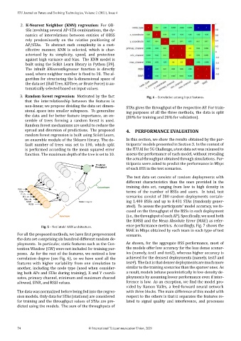
poses. As for the rest of the features, we noticed a low ios (namely, test1 and test2), whereas higher accuracy is
correlation degree (see Fig. 6), so we have used all the achieved for the densest deployments (namely, test3 and
features with higher variability from one simulation to test4). The fact is that denser deployments are much more
another, including the node type (used when consider‑ similar to the training scenarios than the sparser ones. As
ing both APs and STAs during training), X and Y coordi‑ a result, models behave pessimistically in low‑density de‑
nates, primary channel, minimum and maximum channel ployments by assuming lower performance even if inter‑
allowed, SINR, and RSSI values. ference is low. As an exception, we ind the model pro‑
vided by Ramon Vallés, a feed‑forward neural network
The data was normalized before being fed into the regres‑ with three blocks. The main difference of this model with
sion models. Only data for STAs (stations) are considered respect to the others is that it separates the features re‑
for training and the throughput values of STAs are pre‑ lated to signal quality and interference, and processes
dicted using the models. The sum of the throughputs of

74 © International Telecommunication Union, 2021