Page 73 - ITU Journal Future and evolving technologies Volume 2 (2021), Issue 3 – Internet of Bio-Nano Things for health applications

ITU Journal on Future and Evolving Technologies, Volume 2 (2021), Issue 3

The complexity of the local convexity detector
2 800
proposed in [135] is given by O(l) + O(l ), where l is the
length of a convexity metric. O(l) is due to the calcu‑ 700 N =10000
tx
lations of the convexity metric and the threshold, O(l ) -12 2
2
is the complexity due to the moving average operation. 600 D=10 m /s
Further, the computational complexity of maximizing the 500
likelihood in [137] was O(log(N)). This was based on
the Newton‑Raphson method. This technique for detec‑ Number of received molecules, N rx (r, t) 400 r=[1 m, 1.2 m, 1.4 m, 1.6 m, 1.8 m, 2 m]
3
tion was less complex than [118] (complexity is O(S )),
as the CIR reconstruction and threshold determination in 300 t =[0.17 s, 0.24 s, 0.33 s, 0.43 s, 0.53 s, 0.67 s]
every bit interval was not required for detection. Instead 200 peak
authors in [137] used statistical characteristics of the CIR
to estimate the initial distance and set the threshold for all 100
bit intervals in advance for detection. Furthermore, the
0
complexity in [119] was O(S) that is also less than the 0 0.5 1 1.5 2 2.5 3 3.5 4
technique presented in [118]. Time (s)
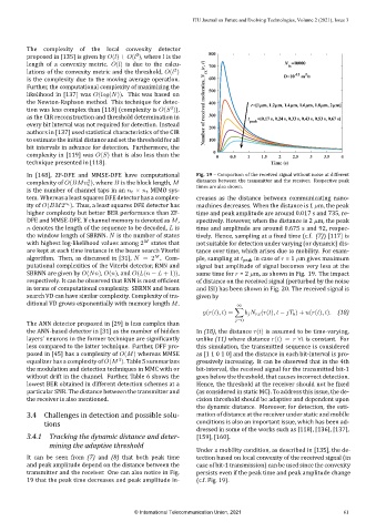
In [148], ZF‑DFE and MMSE‑DFE have computational Fig. 19 – Comparison of the received signal without noise at different
complexity of O(BMn ), where B is the block length, M distances between the transmitter and the receiver. Respective peak
2
t times are also shown.
is the number of channel taps in an n t × n t MIMO sys‑
tem. Whereas a least squares DFE detector has a complex‑ creases as the distance between communicating nano‑
n t
ity of O(BM2 ). Thus, a least squares DFE detector has machines decreases. When the distance is 1 µm, the peak
higher complexity but better BER performance than ZF‑ time and peak amplitude are around 0.017 s and 735, re‑
DFE and MMSE‑DFE. If channel memory is denoted as M, spectively. However, when the distance is 2 µm, the peak
n denotes the length of the sequence to be decoded, L is time and amplitude are around 0.675 s and 92, respec‑
the window length of SBRNN. N is the number of states tively. Hence, sampling at a ixed time (c.f. (7)) [117] is
M
with highest log‑likelihood values among 2 states that not suitable for detection under varying (or dynamic) dis‑
are kept at each time instance in the beam search Viterbi tance over time, which arises due to mobility. For exam‑
M
algorithm. Then, as discussed in [31], N = 2 . Com‑ ple, sampling at t peak in case of r = 1 µm gives maximum
putational complexities of the Viterbi detector, RNN and signal but amplitude of signal becomes very less at the
SBRNN are given by O(Nn), O(n), and O(L(n − L + 1)), same time for r = 2 µm, as shown in Fig. 19. The impact
respectively. It can be observed that RNN is most ef icient of distance on the received signal (perturbed by the noise
in terms of computational complexity. SBRNN and beam and ISI) has been shown in Fig. 20. The received signal is
search VD can have similar complexity. Complexity of tra‑ given by
ditional VD grows exponentially with memory length M.
∞
∑
y(r(t), t) = b j N rx (r(t), t − jT b ) + n(r(t), t). (18)
j=0
The ANN detector proposed in [29] is less complex than
the ANN‑based detector in [31] as the number of hidden In (18), the distance r(t) is assumed to be time‑varying,
layers’ neurons in the former technique are signi icantly unlike (11) where distance r(t) = r ∀t is constant. For
less compared to the latter technique. Further, DFF pro‑ this simulation, the transmitted sequence is considered
posed in [45] has a complexity of O(M) whereas MMSE as [1 1 0 1 0] and the distance in each bit‑interval is pro‑
3
equalizer has a complexity of O(M ). Table 5 summarizes gressively increasing. It can be observed that in the 4th
the modulation and detection techniques in MMC with or bit‑interval, the received signal for the transmitted bit‑1
without drift in the channel. Further, Table 6 shows the goes below the threshold, that causes incorrect detection.
lowest BER obtained in different detection schemes at a Hence, the threshold at the receiver should not be ixed
particular SNR. The distance between the transmitter and (as considered in static MC). To address this issue, the de‑
the receiver is also mentioned. cision threshold should be adaptive and dependent upon
the dynamic distance. Moreover, for detection, the esti‑
3.4 Challenges in detection and possible solu‑ mation of distance at the receiver under static and mobile
tions conditions is also an important issue, which has been ad‑
dressed in some of the works such as [118], [136], [137],
3.4.1 Tracking the dynamic distance and deter‑ [159], [160].
mining the adaptive threshold
Under a mobility condition, as described in [135], the de‑
It can be seen from (7) and (8) that both peak time tection based on local convexity of the received signal (in
and peak amplitude depend on the distance between the case of bit‑1 transmission) can be used since the convexity
transmitter and the receiver. One can also notice in Fig. persists even if the peak time and peak amplitude change
19 that the peak time decreases and peak amplitude in‑ (c.f. Fig. 19).

© International Telecommunication Union, 2021 61