Page 192 - Kaleidoscope Academic Conference Proceedings 2020

2020 ITU Kaleidoscope Academic Conference

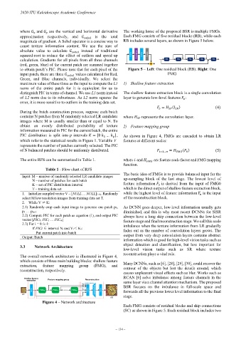
where and are the vertical and horizontal derivative The working horse of the proposed BSR is multiple FMGs.

approximation respectively, and is the total Each FMG consists of five residual blocks (RB), while each
magnitude of gradient. A Sobel operator is a concise way to RB includes several layers, as shown in Figure 5 below.
count texture information content. We use the sum of
absolute value to calculate instead of traditional
squared-root to reduce the effect of outliers and speed up Conv Activation Conv Scale
calculation. Gradients for all pixels from all three channels RB RB RB RB RB
(red, green, blue) of the current patch are summed together +
to obtain patch’s PIC. Please note that for each pixel of the Figure 5 – Left: One residual block (RB). Right: One
input patch, there are three values calculated for Red, FMG
Green, and Blue channels, individually. We select the
maximum value of these three as the input to compute the L1 1) Shallow feature extraction
norm of the entire patch for it is equivalent for us to
distinguish PIC in terms of channel. We use L1 norm instead The shallow feature extraction block is a single convolution
of L2 norm due to its robustness. As L2 norm squares the layer to generate low-level features :

error, it is more sensitive to outliers in the training data set.
= ( ) (4)

During the batch construction process, suppose each batch
contains N patches from M randomly selected LR candidate where represents the convolution layer.
images where M is usually smaller than or equal to N. To
obtain an evenly distributed probability of texture 2) Feature mapping group
information measured in PIC for the current batch, the entire
PIC distribution is split into intervals = [0 … ], As shown in Figure 4, FMGs are cascaded to obtain LR
1

which refer to the statistical results in Figure 1. Variable V features at different scales:
represents the number of patches currently selected. The PIC
of N balanced patches should be uniformly distributed. =1… = ( ) (5)
0
The entire RFS can be summarized in Table 1. where and are feature scale factor and FMG mapping
function.
Table 1 - Flow chart of RFS
The basic idea of FMGs is to provide balanced input for the
Input: M – number of randomly selected LR candidate images
N – number of patches for each batch up-sampling block of the last stage. The lowest level of
K – set of PIC distribution interval feature information is derived from the input of FMG0
0
T – training data set which is the direct output of shallow feature extraction block,
1. Initialize sampled vector V = [NULL … NULL]1×k. Randomly while the highest level of feature information is the input

select M low resolution images from training data set T. of the reconstruction block.
2. While V ≠ K:
2.1) Randomly crop each input image to generate one patch p0, As DCNN goes deeper, low-level information usually gets
p1 … pm-1 diminished, and this is why most recent DCNNs for SISR
2.2) Compute PIC for each patch as equation (1), and output PIC always have a long skip connection between the low-level
vector [PIC0, PIC1 … PICm] feature stage and final reconstruction stage. We call this scale
2.3) For i = 0: k-1: imbalance when the texture information from LR gradually
If PICi ∈ interval Ni and Vi＜ Ki:
Put current patch into batch fades out as the number of convolution layers grows. The
Output: Batch output from very deep convolution layers contains abstract
information which is good for high-level vision tasks such as
3.3 Network Architecture object detection and classification, but less important for
low-level vision tasks such as SR where texture
reconstruction plays a vital role.
The overall network architecture is illustrated in Figure 4,
which consists of three main building blocks: shallow feature
extraction, feature mapping group (FMG), and Many DCNNs, such as [6], [28], [29], [30], could recover the
contour of the objects but lost the details around, which
reconstruction, respectively.
causes unpleasant visual effects such as blur. Works such as
RCAN [6] solve imbalance among feature channels in the
Shallow feature
extraction Feature mapping group Reconstruction same layer via a channel attention mechanism. The proposed
α 0 Spatial attention
α 1 BSR focuses on the imbalance in full-scale space and
Conv FMG 0 FMG 1 FMG N α n Conv Upsampling Conv forwards all the previous lower level information to the final
LR stage.
HR
Figure 4 – Network architecture
Each FMG consists of residual blocks and skip connections
(SC) as shown in Figure 5. Each residual block includes two

– 134 –