Page 191 - Kaleidoscope Academic Conference Proceedings 2020

Industry-driven digital transformation

textures from heavily down-sampled images. Although it can
alleviate the blurring and over-smoothing artifacts to some
degree, its predicted results may not be faithfully
reconstructed and produce unpleasing artifacts [6]. Step0
Down-sample Bicubic/blur-down down-sample
LR dataset HR dataset
RCAN [6] proposed a residual in residual structure to form a Step1
Select image
very deep network of as many as 400 layers which achieves
excellent results. SAN [8] utilizes a novel trainable second- Step2
Select patch
order channel attention module as a substitute for a channel
attention layer in RCAN to adaptively rescale the channel-
wise features. Step3
Calculate PIC
Step4
Qualify patch
Unfortunately, all the works above focus on network Step5
Form balanced batch
structure to achieve better subjective/objective results, and
none of them pay attention to the various imbalance issues BSR training model Loss (Lp + L1 + L2)
presented in this paper. Here, we propose a balanced SR
framework, which we will detail in the next section. Update model & generate No converge?
a new balanced batch
Yes
3. BALANCED SR BSR trained model

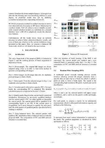
3.1 Architecture Figure 3 – Balanced SR framework

The entire framework of the proposed BSR is illustrated in After one iteration of batch training, if the BSR is not
Figure 3, and the working process of batch acquisition is converged, the current model gets updated and a new
depicted as below: balanced batch is generated using Step 1 to Step 5. The
computation of PIC and BSR network structure is revealed
Step 0: Down-sample. The original HR images are down- later.
sampled using either a bi-cubic or blur-down method to
generate corresponding LR images. 3.2 Random Filter Sampling (RFS)

Step 1: Select images. In LR image data sets, we randomly A traditional neural network training process usually
pick up images to form a batch. involves selecting several LR images randomly from a
specific data set and crop to a fixed size which is called a
Step 2: Select patch. From the selected images in Step 1, we patch in order to form a batch input. The output is the
randomly select patches to form a batch. corresponding high-resolution SR patch. A patch pair can be
described as:
Step 3: Calculate patch information capacity (PIC). For each
batch, the corresponding PIC is computed. The detailed : [ , , , ℎ] → : [ × , × , × , ℎ × ]
calculation process is depicted in Section 3.2 below.
where x and y are the selected patch’s left upper corner
Step 4: Qualify patch. Based on the current batch’s statistical coordinates, and w and h are the patch’s width and height,
distribution (determined by previously qualified batches) accordingly.
and the current patch’s PIC, we either qualify or disqualify
the current patch. The current patch will be qualified if its For each patch, we propose a metric for its information
corresponding batch is not full. If the current patch is measurement, which is called patch information capacity and
disqualified, we’ll move forward to qualify the next patch defined as the following:
until the total number of qualified patches specified in batch
training is satisfied. 2 ℎ−1 −1
= � � � [ ( , , , ℎ)] (1)

Step 5: Form balanced batch. The selected patches with ℎ=0 =0 =0
qualified PIC distribution form a balanced batch to train the
proposed BSR. The computation of PIC and BSR network It represents how much texture information is contained in
structure is revealed later. the patch. The gradient magnitude is calculated by Sobel
operations as follows:

−1 0 +1 +1 +2 +1
0� (2)
= �−2 0 +2� , = � 0 0

−1 0 +1 −1 −2 −1
= | | + | | (3)

– 133 –