Page 193 - Kaleidoscope Academic Conference Proceedings 2020

Industry-driven digital transformation

paths, a residual path which consists of convolution layers
and one activation layer, and an identity path as [25]. Each
FMG is used to estimate a certain scale feature and
contributes to evaluate higher level features by concatenation
of all FMGs’ output to the final reconstruction stage which
shows our balanced multi-scale feature extraction.

3) Reconstruction

All the FMG outputs, as well as the information from a
shallow feature extraction block, are fed into the final
reconstruction block simultaneously:

= ( =1… ) (6)

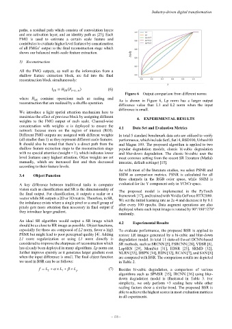
Figure 6 – Output comparison from different norms
where contains operations such as scaling and As is shown in Figure 6, Lp norm has a larger output
reconstruction that are realized by a shuffle operation. difference value than L1 and L2 norm when the input
difference is small.
We introduce a light spatial attention mechanism here to
maximize the effect of previous block by assigning different 4. EXPERIMENTAL RESULTS
weights to the FMG output of each scale. Channel-wise
concatenation with weights α is deployed to ensure the 4.1 Data Set and Evaluation Metrics
network focuses more on the region of interest (ROI).
Different FMG outputs are assigned with different weights In total 5 standard benchmark data sets are utilized to verify
(all smaller than 1) as they represent different scale features. performance, which include Set5, Set14, BSD100, Urban100
It should also be noted that there’s a direct path from the and Magna 109. The proposed algorithm is applied to two
shallow feature extraction stage to the reconstruction stage popular degradation models, classic bi-cubic degradation
with no special attention (weight = 1), which indicates lower and blur-down degradation. The classic bi-cubic uses the
level features carry highest attention. Other weights are set most common setting from the recent SR literature (Matlab
manually, which are increased first and then decreased imresize, default settings) [15].
according to their feature levels.
As with most of the literature studies, we select PSNR and
3.4 Object Function SSIM as comparison metrics. PSNR is calculated for all
three channels in the RGB color space, while SSIM is
A key difference between traditional tasks in computer evaluated for the Y component only in YCbCr space.
vision such as classification and SR is the dimensionality of The proposed model is implemented in the PyTorch
the final output. For classification, it outputs a scalar or a framework [17], and trained with Nvidia GeForce RTX2080.
vector while SR outputs a 2D or 3D matrix. Therefore, in SR, We set the initial learning rate as 2e-4 and decrease it by 0.1
the imbalance exists where a single pixel or a small group of after every 100 epochs. Data augment operations are also
pixels gets more attention than necessary in final output if deployed where each input image is rotated by 90°/180°/270°
they introduce larger gradient. randomly.

An ideal SR algorithm would output a SR image which 4.2 Experimental Results
should be as close to HR image as possible. Object functions,
especially for those are composed of L2 norm, favor a high To evaluate performance, the proposed BSR is applied to
PSNR but might lead to poor perceptual quality [4]. Adding restore LR images generated by a bi-cubic and blur-down
L1 norm regularization or using L1 norm directly is degradation model. In total 11 state-of-the-art DCNN-based
considered to improve the sharpness of reconstruction which SR methods, such as SRCNN [5], FSRCNN [28], VDSR [6],
has already been deployed in many algorithms. Lp norm can LapSRN [29], MemNet [31], EDSR [25], SRMD [32],
further improve sparsity as it generates larger gradient even NLRN [33], DBPN [34], RDN [12], RCAN [7], and SAN [8]
when the input difference is small. The final object function are compared with BSR. The comparison results are depicted
we used in BSR can be as follows: in Table 2.
f = L +α × L + β × L (7) Besides bi-cubic degradation, a comparison of various
1
p
2
algorithms such as SPMSR [35], IRCNN [36] using blur-
down degradation model is illustrated in Table 3. For
simplicity, we only perform ×3 scaling here while other
scaling factors show a similar trend. The proposed BSR is
able to achieve the highest scores in most evaluation matrices
in all experiments.

– 135 –