Page 47 - ITU Journal: Volume 2, No. 1 - Special issue - Propagation modelling for advanced future radio systems - Challenges for a congested radio spectrum

ITU Journal: ICT Discoveries, Vol. 2(1), December 2019

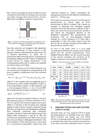
Fig. 7 shows an example of a drop of scatterers from coherence distance . Table 4 summarizes the

a real intersection in Berlin, Germany. Here, the blue, path gain parameters for the different contributions,
red, yellow and gray dots represent first-, second-, where = 20 log ( ).
0
10
0
third-order and diffuse scatterers, respectively.
The model was parameterized and verified against
measurements in various types of street
intersections in Berlin, Germany. Fig. 8 shows an
example of simulated and measured impulse
responses from the intersection outlined in Fig. 7.
The y-axis shows the measurement time and the x-
axis shows the propagation distance of the
multipath components. The measurements are
performed with an ultra-wideband channel
sounder at a center frequency of 5.7 GHz with a
Fig. 7 – Example of scatterers dropped in a simulation area. bandwidth of 1 GHz. The white stripes in the left
Colored dots are specular components, grey dots represent plot are due to the data storage process where no
diffuse scattering. measurements could be taken.
Once the scatterers are dropped in the simulation As seen in the figure there is a very good
area the contribution of each scatterer to the correspondence between the outputs of the channel
impulse response is determined by expressions for: model and the real-life measurements. Some
1) distance dependence, 2) losses due to detailed behavior differs, but the overall structure
interactions with scattering objects, 3) obstructions of the channel evolution and variation of the
by buildings, foliage and other objects, 4) diffraction impulse response is well captured by the GSCM.
around corners, 5) angular dependence of the
scattering interaction, and 6) random, but spatially Table 4 – Path gain parameters for the different multipath
contributions
correlated, large-scale fading.
The transfer function of the channel between any Type Order G0 (dB) dc (m) k (-) Θ (-)
two antennas are calculated as a superposition of all Wall 1st U(−65, −48) U(1, 2) U(2, 8) 1/k
power weighted contributions from the scatterers Wall 2nd U(−70, −59) U(0,1.5) U(1, 6) 1/k
as in (6): Wall 3rd U(−75, −65) U(0, 1) U(1, 4) 1/k
Non- wall 1st U(−68, −52) U(0, 1) U(1, 6) 1/k
( , ) = ∑ =1 − 2 ( ) ( ) (6) Diff. 1st U(−80, −68) U(0, 1) U(1, 1) 1/k

where is the complex antenna amplitude gain in
direction Ω, is the complex amplitude of path l, L

is the total number of paths, is the frequency, and
is the propagation delay, = / . For each MPC

the average path power gain is modeled as in (7):
2
2
̅( ) = ( 0 ) 10 − /10 (7)

2
where is the path propagation distance and is
0
the path power gain at a reference distance of 1 m. Fig. 8 – Measured and simulated impulse responses over time
in the intersection in Fig. 7. The white stripes are due to data
The term describes the path angular power gain, download, with no measurements.
2

which is a function of the incoming and outgoing
2
angles for each scatterer, and is a gain describing 5. BUILDING ENTRY LOSS AND CLUTTER

the effects of obstruction and blockage by buildings. LOSS AT 26 GHz
Each multipath component then undergoes
spatially correlated Gamma distributed large-scale Currently there are two separate ITU-R P-series
fading (with parameters k and θ) so that the Recommendations on building entry loss (BEL),
instantaneous amplitude of each MPC varies around ITU-R P.2109-0 and clutter loss (CL) ITU-R
the mean according to a Nakagami distribution. The P.2108-0. In sharing studies, BEL and CL are treated
autocorrelation of the fading process is described as multiplicative where the overall excess path loss
by a conventional Gudmundson model [12] with is the sum in dB of the individual losses. To assess

© International Telecommunication Union, 2019 31