Page 36 - Proceedings of the 2018 ITU Kaleidoscope

2018 ITU Kaleidoscope Academic Conference

C6 C7 C8 C9 C10
C1 0 1,19 0 0 0
C2 0 0,24 0,71 0 0
C3 1,66 2,14 2,38 0 0
C4 0 0 0 0 0
C5 0,48 0 0,24 0 2,14
C6 0 0 0 0 0
C7 1,66 1,90 0 0,24 0
C8 0 0 0,48 0 0,95
C9 0 0 0 3,33 0
C10 2,38 0 0 0 0
Table 2 shows the distribution of observations among
clusters, and compares the first versus the second execution.
There are five cells with frequencies above 6%, and eight
cells above 5%. Depending on the cutoff, there may be five
or eight stable classes, and this is similar to what we have
interpreted from Figure 1.
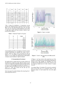
Figure 2 - Clusters’ centroids
Table 3 - Observed F values for K groups.

K F value
2 84,31
3 194,52
4 162,58
5 38,78
6 25,46
7 52,52
8 145,45
9 103,23
10 32,79

Even though the variables in this study do not follow an exact
Gaussian distribution, we estimated the values of the F
statistic. Notice in Table 3 that in all cases the value is
superior to 10. The statistic is below the empirical cutoff
when K=19. We continue the analysis based on the number Figure 3 - Clusters’ centroids between 88 MHz and 108
of clusters determined by the empirical methods. MHz

4.2 Interpretation of the clusters In Figure 2, we have noted at first sight that one of the
clusters, C3, groups the cases of all subscribers who hired the
We performed this analysis with four to seven clusters and Internet service only (usually our subscribers hire both
decided that six would be enough. When varied, we saw broadband access and video services). We continue to plot
on the 3G-downlink band that when there were fewer classes, the frequency bands that are of main interest for ingress
at least one of them grouped mixed patterns. Setting = 7, detection.
the patterns that we identified were the same as the ones seen
with = 6 . The extra cluster did not add any new According to Figure 3, the cluster C4 centroid is consistently
information to the analysis. above all the rest, and C3 is consistently below. In this
frequency range, we could assume there was radio signal
Next, we present the results obtained after executing the k- ingress.
means algorithm with K=6.

– 20 –