Page 35 - Proceedings of the 2018 ITU Kaleidoscope

Machine learning for a 5G future

contains all of the measurements made on the i-th cable

modem, so = { ; ; … ; 4,458 } and = 4,458.

2
1
2
WCSS = ∑ ∑ ∙

=1 =1 After a few attempts to work with the original data, we
decided to standardize each cable modem’s values –that
Where is the size of the cluster k, and is the estimated means that we take each signal strength value, minus the
2

variance of the variable j, in the same cluster. cable modem mean, divided by its standard deviation-. We
found that without standardization, the algorithm would
3.3 Estimation of K catch that some cable modems receive stronger signals,
which may be useful to solve other kinds of problems but not
At the beginning of this section, we assumed that we already to report on signal impairment.
knew the value of K. It is possible -as it happens in this work-
that the value of K is unknown. The WCSS is minimum when 4.1 The search for the value of K
there are as many clusters as observations; therefore, to look
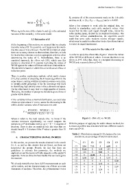
for its absolute minimum is not an appropriate criterion when In order to apply the elbow rule, Figure 1 shows the values
determining the value of K. Nevertheless, there is an of the WCSS at different K values. It seems that there is an
empirical approach, the elbow rule [10], which uses this elbow at K=5. After that, there is a marginal decreasing of
statistic to determine K. It consists in plotting the values of WCSS and a second elbow at K=10.
WCSS against the values of K from which we obtained them.
The decision is based on where the curve shows an elbow or
inflection point.

There is another exploratory method, called stable classes
[11], that consists in executing the k-means algorithm to the
same dataset, starting at different random centers every time,
to identify stable groupings. It has the advantage that leads
to identifying high-density areas in the p-dimensional space.
On the other hand, it may lead to a high number of classes.
Therefore, the number of groups we should keep are those of
greater stable classes.

If the variables follow a Normal distribution, we could also
obtain an approximate F test to assess the decreasing in the
within-cluster variance when K increases one unit:

( ) − ( + 1)
=
( + 1)/( − − 1)

Where n refers to the total sample size. To know if the Figure 1 - Plot of K vs. WCSS
variance decreases significantly, we could compare the
statistic to an F distribution with p; p(n − K − 1) degrees of With the purpose of applying the stable classes method, the
freedom. There is also an empirical rule that says that we k-means algorithm was executed with two different random
should keep K + 1 clusters if the F value is greater than 10 starts and K=10.
[12].
Table 2 - Distribution among K=10 clusters after two
4. CHARACTERIZING SIGNAL INGRESS executions, as percentage of total modem count.

In this section, we present the results obtained in the search C1 C2 C3 C4 C5
for K, as well as the clusters that we found, and how we C1 5,94 7,13 0 6,89 0
interpreted the groups. Despite the fact that there are
guidelines to estimate this parameter, the methods are C2 15,44 0 0,48 1,43 0
exploratory and the decision finally depends on the analyst’s C3 1,66 0 9,03 0 0
expertise. Here we show the best results that we could get to C4 0 11,88 0 0 0
the moment. C5 5,70 2,61 0 0,24 0
C6 0 0 0 0 5,70
We already stated that we have 4,458 measurements on each C7 0 0 0,48 0 0
cable modem, and we interpret every one of them as a new C8 0 0 0 0 2,38
dimension of analysis. Therefore, the p-dimensional vector C9 0 0 0,24 0 0
C10 0 0,71 0 0 0

– 19 –