Page 91 - Proceedings of the 2017 ITU Kaleidoscope

Challenges for a data-driven society

The Buckingham Pi theory is used to find the dimensionless
groups from relevant input and output parameters. The
dimensionality of the original parameters is sharply
decreased and simplified by applying the dimensionless
groups [7]. The major steps to perform the model reduction
with assistance of Buckingham Pi theory are as following:
Step1: Finding the dimension matrix;
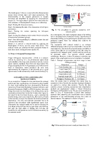
Step2: Determining the rank of the dimensions of full-space
parameters; Fig. 2. The procedures to generate asymptotic drill
Step3: Finding the vectors spanning the full-space reduced model
parameters;
Step4: Finding the reference meta-models which include the As a consequence, the whole asymptotic shape of the drilling
dimensionless parameter groups; hole is calculated and is illustrated. Finally, classification of
sheet metal drilling can be performed by identification of the
Step5: Data-driven modelling by calibration sparse data and parameter region where the drilling hole achieves its
reference meta-models; asymptotic shape.
Schulz et al. derived a reduced model by applying the The asymptotic drill reduced model is an ordinary
Buckingham Pi theory and the steps listed above. This differential equation which can be solved within 1 second for
reduced model can calculate the heat conduction losses in each single run. This fast reduced model makes it possible to
laser sheet metal cutting processes rapidly [8].
collect dense data in an acceptable period. By using the
asymptotic drill reduced model, 10,000 sampling points can
3.4 Proper Orthogonal Decomposition be generated within five seconds without parallel
calculations. However, it takes 30 minutes to produce one
Proper Orthogonal Decomposition (POD) is a numeric sample if the complicated numerical simulation is adopted.
method by searching for a low-dimensional approximate Table 1. Example of parameters and their range in laser
representation of the large scale dynamical systems, such as drilling processes
signal analysis, turbulent fluid flow and large dataset like Parameters Ranges
image processing [9,10]. POD generates a set of orthonormal
basis of dimensions, which minimizes the error from Pulse Duration [tp] 0.1-1.5 [ms]
approximating the snapshots. It can generally give a good Laser Power [PL] 3-10 [kW]
approximation with substantially lower dimensionality [11]. Focal Position [z0] -8-8 [mm]
Beam Radius [w0] 50-350[µm]
4. EXAMPLE FOR LASER DRILLING Rayleigh length [zR] 3-35 [mm]
MANUFACTURING Workpiece Thickness [d] 0.2-5[mm]
As an example to illustrate the data enrichment by reduced After the sparse data is enriched into dense data by
models and data visualization, an advanced reduced model asymptotic reduced model, the machine learning techniques
for sheet metal drilling has been developed by Nonlinear are applied to conduct data analytics. Thereby the data
Dynamics of Laser Manufacturing Processes Instruction and analytics process including appropriate data visualization
Research Department (NLD) in RWTH Aachen University methods are implemented within a Virtual Production
Using this model, the final shape of the drilling holes can be Intelligence (VPI) platform [12]. The process is described in
calculated and described. Inside the formula (see Figure 2), detail in [13]. It implemented a hybrid data analytics
the term F is the local laser fluency, z and x represent the approach with clustering and classification tree to identify
position along z and x axis respectively, the term Fth is based parameters of the manufacturing process that result in
on the heuristic concept of an ablation threshold and material desired outputs. The approach is shown in Figure 3.
dependency. The only one unknown parameter has to be
calibrated and determined with experimental sparse data.
Afterwards, this reduced model can be used to calculate the
final shape of the drilling hole by laser sheet metal drilling.
Not only the final shape of drilling hole but also the
feasibility for each parameter can be indicated accurately by
this reduced model

Fig. 3. Data analytics process to analyze dense data [13]

– 75 –