Page 73 - Kaleidoscope Academic Conference Proceedings 2024

Innovation and Digital Transformation for a Sustainable World

techniques. to encode input features to quantum states, and ansatz (initial
guess) is used in the Quantum circuit, referring real amplitude
Algorithm : PIMA Diabetes Prediction using ML & QML for shaping quantum states as depicted in Figure 5. The
Step 1: ← Load PIMA Diabetes Dataset objective function value over iterations is shown in Figure 6.
Step 2: balanced ← SMOTE( )
Step 3: EDA → balanced
Step 4: reduced ← PCA( balanced )
Step 5: ML and QML Classification Model Selection
Step 6: Model Training and Validation
← Split( reduced )
train , val
← Train( , train )
trained
Validation → trained , val
Step 7: Model Evaluation using Performance Metrics:
Accuracy( ) : ← Accuracy( trained , val )
Figure 6 – Training over iterations.
Precision( ) : ← Precision( trained , val )
Recall( ) : ← Recall( trained , val ) QSVC uses a feature map and kernel that are specified
F1 Score( ) : ← 1_ ( trained , val ) to match the dimensions of the input features for specific
classification problems. The classifier employs quantum
Step 8: Comparative Analysis of Model Performance
computing methods to learn and make accurate predictions.
As the first step, the algorithm takes in the PIMA Diabetes
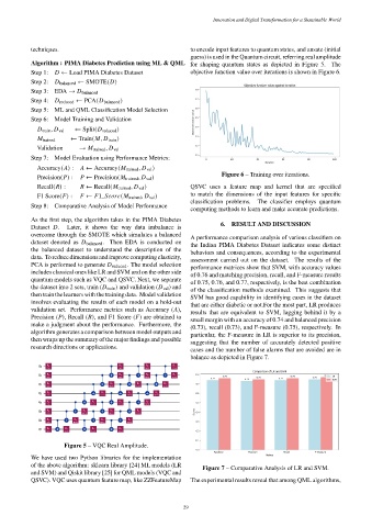
6. RESULT AND DISCUSSION
Dataset . Later, it shows the way data imbalance is
overcome through the SMOTE which simulates a balanced
A performance comparison analysis of various classifiers on
dataset denoted as balanced . Then EDA is conducted on
the Indian PIMA Diabetes Dataset indicates some distinct
the balanced dataset to understand the description of the
behaviors and consequences, according to the experimental
data. To reduce dimensions and improve computing elasticity,
assessment carried out on the dataset. The results of the
PCA is performed to generate reduced . The model selection
performance matrices show that SVM, with accuracy values
includes classical ones like LR and SVM and on the other side
of 0.76 and matching precision, recall, and F-measure results
quantum models such as VQC and QSVC. Next, we separate
of 0.75, 0.76, and 0.77, respectively, is the best combination
the dataset into 2 sets, train ( train ) and validation ( val ) and
of the classification methods examined. This suggests that
then train the learners with the training data. Model validation
SVM has good capability in identifying cases in the dataset
involves evaluating the results of each model on a hold-out
that are either diabetic or not.For the most part, LR produces
validation set. Performance metrics such as Accuracy ( ),
results that are equivalent to SVM, lagging behind it by a
Precision ( ), Recall ( ), and F1 Score ( ) are obtained to
small margin with an accuracy of 0.74 and balanced precision
make a judgment about the performance. Furthermore, the
(0.73), recall (0.73), and F-measure (0.75), respectively. In
algorithm generates a comparison between model outputs and
particular, the F-measure in LR is superior to its precision,
then wraps up the summary of the major findings and possible
suggesting that the number of accurately detected positive
research directions or applications.
cases and the number of false alarms that are avoided are in
balance as depicted in Figure 7.

Figure 5 – VQC Real Amplitude.

We have used two Python libraries for the implementation
of the above algorithm: sklearn library [24] ML models (LR
Figure 7 – Comparative Analysis of LR and SVM.
and SVM) and Qiskit library [25] for QML models (VQC and
QSVC). VQC uses quantum feature map, like ZZFeatureMap The experimental results reveal that among QML algorithms,

– 29 –