Page 327 - Kaleidoscope Academic Conference Proceedings 2024

Innovation and Digital Transformation for a Sustainable World

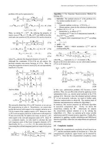
problem (24) can be represented as Algorithm 1 The Gaussian Randomization Method For
Solving (41).
!
¯ v Φ , ¯ v ∗

∑︁
max log 2 (26)a 1: Initialize: The optimal solution ¯ v of the problem (41),
v 1 + Í ¯ v Φ , ¯ v + 2

=1 = +1 the random number Ω and = 1, 2, · · · , Ω.
2: repeat
!
∑︁ 2 3: Generate random vectors q ∼ CN (0, I +1 ).
s.t.¯ v Φ , ¯ v ≥ ¯ v Φ , ¯ v + , ∀ ∈ K (26)b

= +1 4: Obtain random values for the solution of optimization
∗
problem (41) ¯ v = ¯ v · q.
| | = 1, ∀ ∈ N. (26)c
5: Standardize ¯ v to obtain ¯ v .
Then, we define V = ¯ v¯ v . By utilizing the property of

6: Transform ¯ v into × dimensional matrix Θ =

matrix traces ¯ v Φ , ¯ v = Φ , ¯ v¯ v and SDR to forcibly norm
diag ¯ v t N×N matrix.
omit rank-one constraint [25], problem (26) can be relaxed as
7: Compute total computational bits according

! to Θ .

Φ , V
∑︁
max log 2 (27)a 8: ← + 1.
V 1 + Í Φ , V + 2
=1 = +1 9: until = Ω.
10: Output: index which maximizes and its

∑︁
2 corresponding Θ .
s.t. Φ , V ≥ Φ , V + , ∀ ∈ K (27)b ∗

= +1
Í
− Φ
V , = 1, ∀ ∈ {1, · · · , + 1} . (27)c 4 − ∑︁ = +1 Φ , ( , ) , ( , )
= , (31)
ln2 Í 2
V ⪰ 0, (27)d Im V , =1 V = +1 Φ , +
where V , denotes the diagonal elements of matrix V.
where Φ , ( , ) represents ( , ) − ℎ element of Φ , .
Although the constraints (27)b-(27)d are all convex, the
Based on the above derivations, we can reformulate problem
problem remains non-convex because of (27)a. Thus, by
(27) in -th iteration as
using the properties of matrix traces [25], we can equivalently
transform (27)a into max 3 (V) − 4 (V ( −1) )
V
!

Φ , V ∑︁ −1
∑︁
∑︁
log ( −1) 4
2 1 + Í 2 − Re V , − V , ×
=1 = +1 Φ , V + ( −1)

=1 =1 Re V ,
∑︁ ! !
∑︁
= log 2 V Φ , + 2 (28) ∑︁ −1 ( −1) 4
∑︁
=1 = − Im V , − V , × ( −1)
=1 =1
∑︁ ! ! Im V ,
∑︁
− log V Φ , + 2 . (32)a
2
=1 = +1 s.t.(27) − (27) . (32)b
And we define In this case, optimization problem (32) becomes a SDP
problem. Thus, we can efficiently solved by applying convex
! !
∑︁
∑︁
3 (V) = log 2 V Φ , + 2 , optimization tools, e.g., interior point methods or the CVX
=1 = package [24]. However, since the obtained optimal solution
(29)
V is not necessarily rank-one, we need to further apply
! ! ∗
∑︁
∑︁
4 (V) = log V Φ , + 2 . Gaussian randomization to obtain Θ. The detailed steps of
2
=1 = +1 Gaussian randomization are outlined in Algorithm 1.
We can easily obtain that (28) is a DC function, so we can use In summary, this section proposes an AO-based algorithm
DC programming to solve it. Nevertheless, we cannot take to maximize computation rate. Firstly, we derive the
partial derivatives with respect to the complex variables as in closed-form solution for W. Afterwards we achieve
(20) by reason of the complex matrix of V. Moreover, since the closed-form optimal solution of by solving the
4 (V) is not an analytic function, its derivative with respect to subproblem (11). Then, we optimize p by using variable
V does not exist [26]. To address this issue, we derive 4 (V) substitution and SCA-based iterative algorithm. Finally, Θ is
with regard to the real and imaginary parts of V. Since V optimized by applying variable substitution and SDR-based
is a symmetric matrix, we only need to calculate the real iterative algorithm, where the four subproblems are optimized
alternately.
and imaginary parts of the lower triangular elements of V.
Specifically, for , , ≤ , ∀ ∈ N, the partial derivatives
concerning the real and imaginary parts are respectively given 3.5 Complexity Analysis
by
We define the computational complexity of each iteration as
Í
+ Φ , and the maximum number of iterations as . Then, the
4 1 ∑︁ = +1 Φ , ( , ) , ( , )
= , (30) computational complexity upper bound can be denoted by
ln2 Í 2
=1 V = +1 Φ , + O( ). Note that the computational complexity comes
Re V ,
– 283 –