Page 182 - Kaleidoscope Academic Conference Proceedings 2021

2021 ITU Kaleidoscope Academic Conference

see whether the data set contains any incorrect items, and to refined throughout training so that the network transforms
see if it’s acceptable for machine learning[11]. its input in precisely the appropriate ways to generate the
proper output. This is accomplished by sending a sample
of training data into the network, determining how much
the network’s output differs from the correct answer, and
changing the neurons’ internal states to increase the likelihood
of a correct response being produced next time. This results
in a trained network when repeated thousands of times[11].

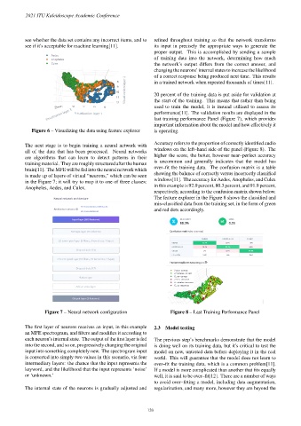
20 percent of the training data is put aside for validation at
the start of the training. This means that rather than being
used to train the model, it is instead utilized to assess its
performance[11]. The validation results are displayed in the
last training performance Panel (Figure 7), which provides
important information about the model and how effectively it
Figure 6 – Visualizing the data using feature explorer is operating.

Accuracy refers to the proportion of correctly identified audio
The next stage is to begin training a neural network with
windows on the left–hand side of the panel (Figure 8). The
all of the data that has been processed. Neural networks
higher the score, the better, however near–perfect accuracy
are algorithms that can learn to detect patterns in their
is uncommon and generally indicates that the model has
training material. They are roughly structured after the human
over–fit the training data. The confusion matrix is a table
brain[11]. The MFE will be fed into the neural network which
showing the balance of correctly versus incorrectly classified
is made up of layers of virtual “neurons," which can be seen
windows[11]. The accuracy for Aedes, Anopheles, and Culex
in the Figure 7; it will try to map it to one of three classes:
in this example is 92.9 percent, 80.3 percent, and 91.9 percent,
Anopheles, Aedes, and Culex.
respectively, according to the confusion matrix shown below.
The feature explorer in the Figure 8 shows the classified and
mis–classified data from the training set, in the form of green
and red dots accordingly.

Figure 7 – Neural network configuration Figure 8 – Last Training Performance Panel

The first layer of neurons receives an input, in this example 2.3 Model testing
an MFE spectrogram, and filters and modifies it according to
each neuron’s internal state. The output of the first layer is fed The previous step’s benchmarks demonstrate that the model
into the second, and so on, progressively changing the original is doing well on its training data, but it’s critical to test the
input into something completely new. The spectrogram input model on new, untested data before deploying it in the real
is converted into simply two values in this scenario, via four world. This will guarantee that the model does not learn to
intermediary layers: the chance that the input represents the over–fit the training data, which is a common problem[11].
keyword, and the likelihood that the input represents ‘noise’ If a model is more complicated than another that fits equally
or ‘unknown.’ well, it is said to be over–fit[12]. There are a number of ways
to avoid over–fitting a model, including data augmentation,
The internal state of the neurons is gradually adjusted and regularization, and many more, however they are beyond the

– 120 –