Page 98 - ITUJournal Future and evolving technologies Volume 2 (2021), Issue 1

ITU Journal on Future and Evolving Technologies, Volume 2 (2021), Issue 1

On the Monte Carlo window in Fig. 6, we have speci ied • Model 3: We cut the message on 5 times when we
the BERTool parameters (which are detailed in Table 1) are coding with Hamming coding rate = 11/15.
2
based on our scenarios. In order to generate BER data for Since in Model 3, the Hamming code has length 75
each communication system using the Simulink models, and dimension 55, we have to append 5 zeros to 50
we follow ive steps based on the following BERTool pro‑ information bits before encoding.
cess [15]:

1. We calculate Bit Error Rate (BER) as a function of the Model 1: Simple Hamming code [63, 57]
energy per bit to noise power spectral density ratio
( ).
0
6
2. We ix the number of errors ( = 10 ) and the
10
number of bits ( = 10 ) in order to make ac‑
curate error rate. We have chosen this number of
bits value to prevent the simulation from running too
long, especially at large values of .
0
3. We have speci ied the range based on our PLC
0 (a)
channel model: = 0 ∶ 15 dB.
0
0
10
4. We generate the BER data for a chosen Simulink
model. This Simulink Model is displayed and run in Model 1: Hamming CR 5
10 -1
real time on the models being simulated window (as Fit Model 1
shown in Fig. 6) for each value of the energy per bit
10 -2
to noise ratio . BERTool iterates over our choice of
0
the energy per bit to noise ratio value and collects BER 10 -3
0
the results on a list of simulations.
10 -4
5. Finally, we run the simulation in order to plot the es‑
timated BER values function of the previous steps. -5
10
The plot of simulation window is displayed and
shows each curve for each Simulink model. We save
10 -6
later in the list of simulations each curve in order to 0 2 4 6 8 10 12
compare graphically the different models. E /N (dB)
0
b
(b)
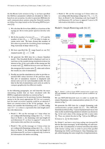
In the following paragraphs, we will describe the most Fig. 7 – Model 1: (a)Short‑frame OFDM communication model using
interesting models that we have simulated with the MATLAB‑Simulink tools (b) BER performance plotted on BERTool ap‑
BERTool application interface as shown in Fig. 6. plication
As we have discussed in the previous Section, Hamming We use MATLAB‑Simulink tools in order to model the
seems to be the most appropriate ECC for our scenario, simple Hamming code communication system [63, 57] as
but the small correction capacity could be an obstacle if shown in Fig. 7.
there are several errors in the 50 bit package. For in‑
stance, we consider the Hamming code [ , ] with coding We generate the BER data for a simple Hamming code
rate = / where represents the code length and communication system model [63, 57]. This MATLAB‑
the code dimension. Simulink model (see Fig. 7 (a)) is displayed and run in real
time on the models being simulated window (as shown in
• Model 1: We cut the message on 1 time when we Fig. 6) for each value of the energy per bit to noise ratio
are coding with Hamming coding rate = 57/63; . Then, we obtain the plot in Fig. 7 (b) as the BER per‑
5
0
Since in Model 1, the Hamming code has length 63 formance vs. for this model.
and dimension 57, we have to append 7 zeros to 50 0
information bits and then do encoding. For Model 1, we have a very long coding rate (around 50
bits for the input message). In the following, we will com‑
• Model 2: We cut the message on 2 times when we pare to the concatenation of several encoders/decoders
are coding with Hamming coding rate = 26/31; with shorter coding rates in order to prove that parallel
4
Since in Model 2, the Hamming code has length 62 Hamming has better performances than Hamming sim‑
and dimension 52, we have to append only 2 zeros to ple, while keeping the same simplicity of implementation.
50 information bits before encoding.

82 © International Telecommunication Union, 2021