Page 67 - ITUJournal Future and evolving technologies Volume 2 (2021), Issue 1

ITU Journal on Future and Evolving Technologies, Volume 2 (2021), Issue 1

This is followed by the computation of the average Algorithm 3 Johnson’s Algorithm
intra‑cluster propagation latency variation (intraClusVar Require: ( , ) {undirected weighted network graph}
denoted by ( ) in Eq. (3)) between the switches 1: Compute ℎ [ ] ← [ ] ∪ { is a new
′
′
′

(Instruction 4). Next a reference data set ( graph containing }
denoted by in Eq. (4)) of the network topology 2: for ∈ [ ] {for all switches ( ) in the original
is randomly generated (Instruction 6). The average graph} do
intra‑cluster latency variation of the reference data set 3: [ ] ← [ ] ∪ ( , ) ∶ ∈ [ ]
′
∗
(intraClusVarRef denoted by ( ) in Eq. (4)) is 4: ( , ) ← 0

computed (Instruction 7). The Gap Statistics is calculated 5: end for
using Eq. (3) and (4). Finally, the standard deviation of 6: if − ( , ) == then
′
B Monte Carlo replicates is calculated [30]. The optimal
7: print Error! Negative cycle detected.
number of controllers is one that meets the condition in 8: else
Eq. (5), where +1 denotes the standard deviation of B 9: for ∈ [ ] do
Monte Carlo replicates.
10: set ℎ( ) ← ( , ) compute shortest path using
Bellman‑Ford
∗
∗
( ) = ( ( )) − ( ( )) (3) 11: end for

′
12: for ( , ) ∈ [ ] do
13: ← ( , ) + ℎ( ) − ℎ( )
where 14: end for
15: for ∈ [ ] do
1 16: execute ( , , ) to compute
∗
∗
∗
( ( )) = ( ( )) (4)

( , ) for all ∈ [ ]
17: for ∈ [ ] do
18: ( , ) ← ( , ) + ℎ( ) − ℎ( )
( ) ≥ ( + 1) − +1 (5) 19: end for
20: end for
4.3 Optimal controller location 21: end if
22: return shortest path matrix
This section describes the algorithms used to ind the best
locations to place SDN controllers.
4.3.2 Partition around medoids (PAM)
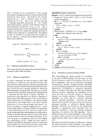
4.3.1 Johnson’s algorithm After determining the optimal number of controllers
to use given a WAN topology, the next step is to ind
In order to determine the best locations to place SDN the best locations to place the controllers such that the
controllers in a WAN, the shortest paths between each QoS is maximized. This can be achieved by leveraging
pair of switches must be known. Johnson’s algorithm [39] ”unsupervised” machine learning heuristic algorithms
provides a means to ind the shortest paths between node (such as Simulated Annealing [41] and Clustering LARge
pairs and has become a popular method for addressing Applications (CLARA)[42]) or exhaustive algorithms
SDN optimization problems [40]. Therefore, we used the (such as k‑means [43] [44] and PAM [45] [46][47].
results from this algorithm alongside the PAM algorithm However, heuristic algorithms are suboptimal in the
to determine the best places to deploy controllers. A sense that they are primarily focused on optimizing
pseudocode of this algorithm is as shown in Algorithm 3 runtime over solution accuracy. Therefore, heuristic
and consists of the following steps: First a new arbitrary algorithms are more ideal for scenarios requiring
switch (denoted by ) is added to the network graph, dynamic controller placement. However, this study
connected by zero‑weight links to all other switches explores static controller placement, where the controller
(denoted by ) in the network graph (Instructions 1‑5). placement problem is addressed during network
If this step detects a negative weight‑cycle (i.e. a cycle planning. Therefore, the accuracy of the optimization
whose weight sums to a negative number), the algorithm algorithm is signi icantly more important than the
is terminated (Instruction 6‑7). Second, a single source speed of computation. From the available exhaustive
shortest path algorithm called Bellman‑Ford algorithm is algorithms, we opted for the PAM algorithm. This is
evoked, to ind the shortest path ℎ( ) from each switch mainly because the k‑means algorithm is very sensitive
in the network to the new switch (Instructions 9‑11). to outliers which can lead to solution inaccuracy [48].
Next, the graph is reweighted to ind new link weights Unlike k‑means, PAM is more stable and more accurate
(Instruction 12‑14). Finally, the new switch is [49].
removed, and Dijkstra’s algorithm is used to compute the Algorithm 4 describes the steps we followed to compute
shortest paths ( , ) from each each node to every other the optimal locations of SDN controllers. Our approach
node in the reweighted graph (Instructions 15‑22). assumes co‑location of controllers and switches. First,

© International Telecommunication Union, 2021 51