Page 21 - ITU Journal Future and evolving technologies Volume 2 (2021), Issue 4 – AI and machine learning solutions in 5G and future networks

ITU Journal on Future and Evolving Technologies, Volume 2 (2021), Issue 4

mation is the current path state. For the irst cell of the 4.7 Neurons
gated recurrent unit (GRU), the information of the irst
link of a path is being used as the input. Then, the re‑ The inal path state information is obtained through the
sult of this irst calculation, and the information of the message passing [2] loop. This inal information is mainly
second link is used in the next step. This is done until used for predicting the average delays in two steps, one
all link information of a path has been used. This works neural network with two hidden layers each with 8 neu‑
well as long as no heterogeneous queuing is in the data. rons. The other neural network does not contain an acti‑
However, to tackle the additional complexity of queuing, vation function and is described in Step 4.4. As we have
we decided to use two gated recurrent networks stacked increased the dimension of this path state information in
the previous step from 32 to 128, it may be useful to in‑
together. The idea of using stacked gated recurrent net‑
crease the number of neurons in the irst neural network
works has already been used in a slightly different con‑
responsible for prediction. The baseline number of neu‑
text [23], where neural networks predicted traf ic volume
rons is 8. We increased this number to 128 and 256 and
in road networks to relieve traf ic congestion. Further‑
more, these gated recurrent networks seemingly allow observed that there is no signi icant difference between 8,
for more lexibility as more parameters can be trained. 128 or 256 neurons. The results for 128 and 256 neurons
The average error for this Step 5 is about 3.18% (95% CI are given in Table 1 as Step 7A and Step 7B with an av‑
[2.94%, 3.41%]); see Table 1. erage error of 1.61% and 1.67%, respectively. As already
mentioned, there is no difference to 8 neurons under Step
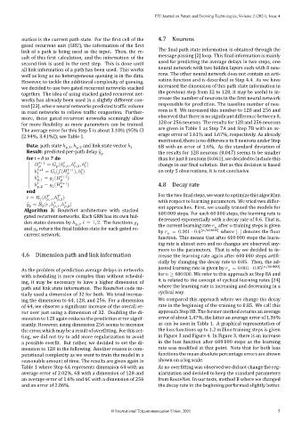
Data: path state ℎ ,1 , ℎ ,2 and link state vector ℎ 6B with an error of 1.6%. As the standard deviation of
Result: predicted per‑path delay ̂ the results for 128 neurons (0.047) seems to be smaller
for t = 0 to T do than for just 8 neurons (0.061), we decided to include this

+1 = (ℎ ,1 , ℎ ,2 , ℎ ) change in our inal solution. But as this decision is based

ℎ +1 = ( ( +1 ), ℎ ) on only 5 observations, it is not conclusive.

ℎ ,1 = ( +1 )
1
ℎ ,2 = ( +1 ) 4.8 Decay rate
1
end
= (ℎ , ℎ ) For the two inal steps, we want to optimize this algorithm
1
,1
,2
̂ = ( , ℎ , ℎ ) with respect to learning parameters. We tried two differ‑
2 ,1 ,2 ent approaches. First, we usually trained the models for
Algorithm 3: RouteNet architecture with stacked 600 000 steps. For each 60 000 steps, the learning rate is
gated recurrent networks. Each GRN has its own hid‑ decreased exponentially with a decay rate of 0.6. That is,
den states denotes by ℎ , = 1, 2. The functions 1 the current learning rate after training steps is given
,

and return the inal hidden state for each gated re‑ by = 0.001 ⋅ 0.6 ⌊ /60 000⌋ where ⌊.⌋ denotes the loor
2
current network.
function. This means that after 600 000 steps the learn‑
ing rate is almost zero and no changes are observed any‑
more to the parameters. That is why we decided to in‑
4.6 Dimension path and link information crease the learning rate again after 600 000 steps arti i‑
cially by changing the decay rate to 0.85. Then, the ad‑
justed learning rate is given by = 0.001 ⋅ 0.85 ⌊ /60 000⌋
As the problem of prediction average delays in networks
with scheduling is more complex than without schedul‑ for ≥ 600 000. We refer to this approach as Step 8A and
ing, it may be necessary to have a higher dimension of it is related to the concept of cyclical learning rates [24]
path and link state information. The RouteNet code ini‑ where the learning rate is increasing and decreasing in a
tially used a dimension of 32 for both. We tried increas‑ cyclical way.
ing the dimension to 64, 128, and 256. For a dimension We compared this approach where we change the decay
of 64, we observe a signi icant increase of the overall er‑ rate in the beginning of the training to 0.85. We call this
ror over just using a dimension of 32. Doubling the di‑ approach Step 8B. The former method returns an average
mension to 128 again reduces the prediction error signif‑ error of about 1.47%, the latter an average error of 1.36%
icantly. However, using dimension 256 seems to increase as can be seen in Table 1. A graphical representation of
the error, which may be a result of over itting. For this set‑ the loss functions up to 1.2 million training steps is given
ting, we did not try to add more regularization to avoid in Figure 3 and Figure 4. In Figure 3, there is an increase
a possible over it. But rather, we decided to set the di‑ in the loss function after 600 000 steps as the learning
mension to 128 in the following. Another reason is com‑ rate was modi ied at that point. Note that for both loss
putational complexity as we want to train the model in a functions the mean absolute percentage errors are shown
reasonable amount of time. The results are given again in shown on a log scale.
Table 1 where Step 6A represents dimension 64 with an As no over itting was observed we did not change the reg‑
average error of 2.02%, 6B with a dimension of 128 and ularization and decided to keep the standard parameters
an average error of 1.6% and 6C with a dimension of 256 from RouteNet. In our tests, method B where we changed
and an error of 2.86%. the decay rate in the beginning performed slightly better.

© International Telecommunication Union, 2021 5