Page 20 - ITU Journal Future and evolving technologies Volume 2 (2021), Issue 4 – AI and machine learning solutions in 5G and future networks

ITU Journal on Future and Evolving Technologies, Volume 2 (2021), Issue 4

there are also three weights for the policies WFQ and DRR. information is now used as input. The average error is
For the policy SP, we arti icially set these three weights to about 4.46% (95% CI [3.97%, 4.94%]) as can be seen un‑
1. der Step 3 in Table 1.
For the scheduling policy, we used dummy variables,
since there are three different policies. Let e =
3
′
( , , ) ∈ ℝ be the th canonical vector with = 4.4 Residual connection
1
3

2
′
1 if = and = 0 otherwise. Note that denotes the

transpose of . For simplicity, the scheduling policy is For the readout neural network, we used a similar idea

identi ied as integers 0, 1 or 2. Then the dummy variable already used in the original RouteNet model [3]. They
for the scheduling policy can be written as +1 (some‑ used a residual connection for the path information to
times known as ”one hot” encoding). the last hidden layer of the readout neural network. This
For this particular data set there is exactly one low for can be seen as some kind of residual neural network [21].
each path as already mentioned in Section 3. Hence, we However, this idea is not present in the RouteNet code
can identify paths with lows and can therefore assign provided for the challenge. The readout neural network
each path a ToS. That is why we can use ToS as path in‑ consists of two hidden layers. The output of this neural
formation. Other variables for the path information are network together with the inal path state information is
the average data rate on that path (AvgBw), the gener‑ used as input in a second neural network with one hid‑
ated packets (PKtsGen), average bit rate per time unit den layer and without any activation function (which is
(EqLambda), average number of packets of average size equivalent to a linear activation function) as the path state
generated per time unit (AvgPktsLambda), information information can be important for estimating the average
about packet sizes (AvgPktSize, PktSize1, PktSize2) delays. The number of neurons for this layer is chosen to
and a variable describing the upper limit for the inter‑ be equal to the dimension of the input.
packet arrival times used in the OMNeT++ simulation The results are similar to the earlier results. The average
(ExpMaxFactor). All these variables were as well shifted error for Step 4 is about 4.55% (95% CI [4.38%, 4.71%]).
into [0, 1] to improve the stability of the model. However, the standard deviation is reduced by a factor of
We decided to split the average desired data rate on a path about 3 = 0.39/0.13, which means the results are stabler,
(AvgBw) into different variables for each ToS, respectively. which can be explained by this residual neural network.
For example, if the ToS is 1, then the irst of these three There are hypotheses that such neural networks smooth
variables contains the average data rate, while the other the loss function and the algorithm does get stuck less of‑
two are set to 0. For illustration, let ∈ ℝ , ∈ {0, 1, 2} ten in non‑optimal local minima [21][22].
≥0
be the data rate and ToS, where the ToS is identi ied by To illustrate this modi ication, we refer to the pseudo
integers. Then this data rate dummy variable can be writ‑ code 2. In contrast to the unmodi ied code 1, the readout
ten as ⋅e +1 . We also used ToS additionally for the initial neural network is separated into two feed forward neu‑
path state information. It should be noted that many of ral networks. The output of the irst neural network with
those variables listed above are highly correlated. How‑ two hidden layers and ”relu” activation functions is used
ever, we did not encounter any problems and decided to as input for the second neural network. Note that the path
keep these variables without any further modi ication. By state information is used in both neural networks as in‑
adding these additional variables, we now take into ac‑ put.
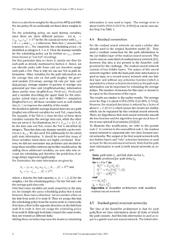
count the scheduling and therefore the prediction of av‑ Data: path state ℎ and link state vector ℎ

erage delays improved signi icantly. Result: predicted per‑path delay ̂
For illustration, the state information are given by
for t = 0 to T do
+1

′

ℎ = [ , , , , ′ +1 , 0, … , 0] ∈ ℝ 32 and +1 = (ℎ , ℎ )

2
3
1

+1
32
′

ℎ = [ ⋅ ′ +1 , … , 0] ∈ ℝ , ℎ = ( ( ), ℎ )

ℎ +1 = ( +1 )

where denotes the link capacity, ( = 1, 2, 3) for the end

weights, for the scheduling policy, for the ToS and for = (ℎ )
1

the average path data rate. ̂ = ( , ℎ )

2
Note that some variables are node properties in the data Algorithm 2: RouteNet architecture with modi ied
set, for example the queue scheduling policy that is used. readout neural network
However, lows have a direction. Let us consider a low on
the link from node A to node B. Then we assign this link
the scheduling policy from the source node A. Conversely, 4.5 Stacked gated recurrent networks
if we have a low in the opposite direction on the link from
node B to node A, then we assign the scheduling policy The idea of the RouteNet architecture is that for each
from node B. Although both links connect the same nodes, path/ low we have information about all links of which
they are treated as different links. the path consists. And this link information is used as in‑
Adding these variables improves the model as scheduling put in a gated recurrent neural network. The initial infor‑
4 © International Telecommunication Union, 2021