Page 163 - ITU Journal Future and evolving technologies – Volume 2 (2021), Issue 2

ITU Journal on Future and Evolving Technologies, Volume 2 (2021), Issue 2

3 0.14
Multi-rotor UAVs Multi-rotor UAVs
Helicopters Helicopters
2.5 Fixed wing UAVs 0.12 Fixed wing UAVs
Small fixed wing planes Small fixed wing planes
Large fixed wing planes Large fixed wing planes
2 Fighter jets 0.1 Fighter jets
Cruise missiles 0.08 Cruise missiles
PDF 1.5 Birds PDF Birds
Ballistic missiles
Ballistic missiles
Rockets & artillery
HGVs 0.06 Rockets & artillery
HGVs
1
0.04
0.5
0.02
0 0
0 10 20 30 40 50 60 70 80 0 1000 2000 3000 4000 5000 6000 7000 8000
Length of central part (m) Max. velocity (m/s)
(a) (b)
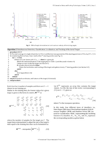
Fig. 8 – PDFs of length of central section and maximum velocity of the training targets.

Algorithm 2 Simultaneous Detection, Classi ication, Localization, and Tracking of the Aerial Target.
1: procedure SDCLT
2: % The total coverage of a single virtual door is Δ ℎ and the total area spanned at all the steering positions is Δ Δ (2 +1) ℎ
th
3: % Considering that we have laser mesh at the steering position (see Fig. 3 )
4: for i = ‑N:N do
5: if there are laser beams with / < then for a given pfa
G
6: Obtain the estimated features of the target given in Table 1, (and discussed in Section 4)
7: Categories and classify the target (see Section 5)
8: if a positive threat identi ied then
th
9: Obtain the localization and tracking of the target and update at every steering position (see Section 5.2)
10: end if
11: else
12: Steering positions only
13: end if
14: end for
15: return Estimated coordinates, and features of the target (if detected)
16: end procedure

Each class has number of samples and there are = 11 Let C (Tr) represents an array that contains the target

classes in our training set. classes. In (14), the size of this vector corresponding to
Similar to the training data, the feature values for a given (11) are × , given as
target is given in the form of a matrix, M (eval) as
[ 1,1 1,2 … 1, 2,1 2,2 …
(Tr)
(c) (c) ℎ (c) (w) (w) (t) C = … … … ]
1
1
1
1
1
1
⎡ (c) (c) (c) (w) (w) (t) 2, ,1 ,2 ,

⎢ 2 2 ℎ 2 2 2 2 (14)
⎢ ⋮ ⋮ ⋮ ⋯ ⋮ ⋮ where is the transpose operation.
(c) (c) (c) (w) (w) (t)

M (eval) = ⎣ ′ ′ ℎ ′ ′ ′ ′ (12)

(t) 1 1 1 ℎ (G) In this study, four different types of iers, i.e.,

1
1
(t) 2 2 2 ℎ (G) ⎤ Naive Bayes (NB, Linear Discriminant Analysis (LDA, K‑
2 ⎥
2

⋮ ⋮ ⋮ ⋮ ⋮ ⎥ nearest Neighbor (KNN, and Random Forest (RF, are
(t) (G) used for classi ication. With representing the modeling

′ ′ ′ ′ ℎ ′ ⎦

function of a classi ier, ℳ , ℳ , ℳ , and ℳ expresses

4
1
2
3
the corresponding models as given below
′
where the number of samples for the target are . The
target data is interpolated to adjust the size of the target’s
data equal to the training data that can be formulated as
M (eval) =interpolate(M (eval) , ). (13)
© International Telecommunication Union, 2021 149