Page 212 - Kaleidoscope Academic Conference Proceedings 2020

2020 ITU Kaleidoscope Academic Conference

The displacement of the body is computed by dividing the 3.3 Skeleton Generation and Processing
displacement of the neck by height H. The normalized joint
positions are obtained by normalization using the body The human skeleton is generated by using a stacked
height H. The displacement of the joints is computed using hourglass network. This neural network is used to detect
the normalized coordinate and it has 13 joints multiplied by human skeleton (joint positions) from each video frame, and
2 displacements per joint to give a 104 dimension for N=5 then the skeleton is utilized as raw data to extract features
frames. and make classification by using machine-learning
algorithms [12].
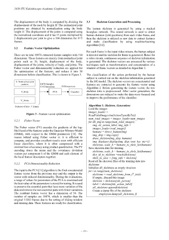
3.2 Feature Vector Optimization
For each frame in the input video stream, the human subject
There are in total 10874 extracted feature samples with 314 is detected and the skeleton for frame is generated. Hence for
dimensions. These features are mainly from normalized joint a video stream, continuous sequence of skeleton information
points such as Xs, height, displacement of the body, is generated. The skeleton vectors are processed by various
displacement of the joints, velocity of body, and joints. The techniques such as transformations and concatenation of a
Fisher vector and dimensionality reduction are applied for window of frame vectors as detailed in Algorithm 1.
the optimization of the features, and reduce it into 50
dimensions before classification. This is shown in Figure 3. The classification of the action performed by the human
subject is carried out on the skeleton information generated
X: Normalized joint by the HG model. The skeleton vectors are concatenated and
position 10874 Samples features are extracted to generate the feature vector using
314 Dimensions 50 Dimensions Algorithm 2. Before generating the feature vector, the raw

V_body PCA Classifier skeleton data is preprocessed. After vector generation, the
dimensions are reduced to make the data more focused and
to improve the performance of the classifier.
V_Joints
Algorithm 1: Skeleton_Generation:
Features of prev. 5 frames
Load the images
images_loader =
Figure 3 - Feature vector optimization ReadValidImagesAndActionTypesByTxt()
num_total_images = images_loader.num_images
3.2.1 Fisher Vector for ith_img in range(num_total_images):
img, str_action_label, img_info =
The Fisher vector (FV) encodes the gradients of the log- images_loader.read_image()
likelihood of the features under the Gaussian-Mixture-Model humans = detect_human(img)
(GMM), with respect to the GMM parameters [10]. The img_disp = img.copy()
reason behind using Fisher vector is: it is efficient to draw_skeleton(img_disp, humans)
compute, and provides excellent results even with efficient img_displayer.display(img_disp, wait_key_ms=1)
linear classifiers, where it is often compressed with a skeletons, scale_h = humans_to_skels_list(humans)
minimal loss of accuracy using product quantization. The FV Save skeleton data for training
encoding stores the mean and the covariance deviation skeletons, scale_h = humans_to_skels_list(humans)
vectors per component k of the GMM and each element of dict_id_to_skeleton =track(skeletons)
the local feature descriptors together. skels_to_save = [img_info + skeleton]
Read all the skeleton files of the training data into
3.2.2 PCA Dimensionality Reduction skeletons
Initialize all_skeletons as empty structure
The input to the PCA [11] algorithm is the final concatenated for i in range(num_skeletons):
feature vector from the previous step and the output is the skeletons = read_skeletons_from_i _txt(i)
th
vector with reduced dimensionality. During the evaluations, If empty, discard this image
a range of values for parameters of the PCA is examined and skeleton = skeletons[idx_person]
the best value of the parameters is stored for testing. It is used label = skeleton[idx_action_label]
to preserve the essential parts that have more variation of the all_skeletons.append(skeleton)
data and remove the non-essential parts with fewer variations. Create a dump file of the skeleton
The resultant feature vector has a dimension of 50. The simplejson.dump(all_skeletons, f)
number of samples are 10874, which is smaller than the
original 11202 frames due to the setting of sliding window
and missing data. These features are ready for classification.

– 154 –