Page 213 - Kaleidoscope Academic Conference Proceedings 2020

Industry-driven digital transformation

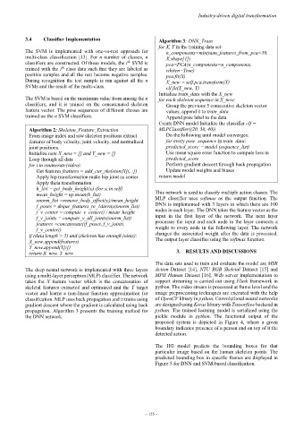
3.4 Classifier Implementation Algorithm 3: DNN_Train
for X, Y in the training data set:
The SVM is implemented with one-vs-rest approach for n_components=min(num_features_from_pca=50,
multi-class classification [13]. For n number of classes, n X.shape[1])
th
classifiers are constructed. Of these models, the i SVM is pca=PCA(n_components=n_components,
th
trained with the i class data such that they are labeled as whiten=True)
positive samples and all the rest become negative samples. pca.fit(X)
During recognition the test sample is run against all the n X_new = self.pca.transform(X)
SVMs and the result of the multi-class. clf.fit(X_new, Y)
Initialize train_data with the X_new
The SVM is based on the maximum value from among the n for each skeleton sequence in X_new:
classifiers, and it is trained on the concatenated skeleton Group the previous 5 consecutive skeleton vector
feature vector. The pose sequences of different classes are values, append it to train_data
trained on the n SVM classifiers. Append pose label to the data
Create DNN model Initialize the classifier clf =
Algorithm 2: Skeleton_Feature_Extraction MLPClassifier((20, 30, 40))
From image index and raw skeleton positions extract Do the following until model converges:
features of body velocity, joint velocity, and normalized for every pose_sequence in train_data:
joint positions. predicted_score = model (sequence_list)
Initialize new X_new = [] and Y_new = [] Use mean square error function to compute loss in
Loop through all data predicted_score
for i in enumerate(video): Perform gradient descent through back propagation
Get features features = add_cur_skeleton(X[i, :]) Update model weights and biases
Apply hip transformation make hip joint as center return model
Apply theta transformation
h_list = get_body_height(xi) (for x i in self)
mean_height = np.mean(h_list) This network is used to classify multiple action classes. The
xnorm_list =remove_body_offset(xi)/mean_height MLP classifier uses softmax as the output function. The
f_poses = deque_features_to_1darray(xnorm_list) DNN is implemented with 3 layers in which there are 100
f_v_center = compute_v_center() / mean_height nodes in each layer. The DNN takes the feature vector as the
f_v_joints = compute_v_all_joints(xnorm_list) input in the first layer of the network. The next layer
features =concatenate((f_poses, f_v_joints, processes the input and each node in the layer connects a
f_v_center)) weight to every node in the following layer. The network
if (data length > 5) and (skeleton has enough joints): changes the associated weight after the data is processed.
X_new.append(features) The output layer classifies using the softmax function.
Y_new.append(Y[i])
return X new, Y new 3. RESULTS AND DISCUSSIONS

The data sets used to train and evaluate the model are MSR
The deep neural network is implemented with three layers Action Dataset [14], NTU RGB Skeletal Dataset [15] and
using a multi-layer perceptron (MLP) classifier. The network MPII Human Dataset [16]. Web server implementation to
takes the X feature vector which is the concatenation of support streaming is carried out using Flask framework in
skeletal features extracted and optimized and the Y target python. The video stream is processed at frame level and the
vector and learns a non-linear function approximation for image preprocessing techniques are executed with the help
classification. MLP uses back propagation and it trains using of OpenCV library in python. Convolutional neural networks
gradient descent where the gradient is calculated using back are designed using Keras library with Tensorflow backend in
propagation. Algorithm 3 presents the training method for python. The trained learning model is serialized using the
the DNN network. pickle module in python. The functional output of the
proposed system is depicted in Figure 4, where a green
boundary indicates presence of a person and on top of it the
detected action.

The HG model predicts the bounding boxes for that
particular image based on the human skeleton points. The
predicted bounding box in specific frames are displayed in
Figure 5 for DNN and SVM-based classification.

– 155 –