Page 133 - ITU Journal, Future and evolving technologies - Volume 1 (2020), Issue 1, Inaugural issue

ITU Journal on Future and Evolving Technologies, Volume 1 (2020), Issue 1

method. Moreover, the weights k of the target NN is worth mentioning that the focus of the results is
-
are updated with the weights of the evaluation NN put on the temporal variations of the offered load so,
every M time steps. The reader is referred to [33] from the spatial perspective, it is assumed, for
for details on the mathematical formulation of this simplicity, that the aggregate offered load is
process. homogeneously distributed across the cells.

The training process stops after a sufficient number Table 1 – SLA parameters
of time steps that ensures the convergence of the GSM GST
process. At this point, the ML training host is ready Attributes MNO1 MNO2
to provide the evaluation NN parameters k so that
the model can be applied on the real network using dlThptPerSlice 6 Gb/s 4 Gb/s
the ML inference host. termDensity 1000 UEs/km 2 500 UEs/km 2
dlThptPerUe 50 Mb/s 100 Mb/s
5. ILLUSTRATIVE SCENARIO AND Table 2 – Cell configuration
EVALUATION
Parameter Value
To illustrate the behavior the proposed cross-slice
optimization framework and ML-assisted solution, Number of cells 5
let us consider a scenario with a localized RAN Cell radius 100m
deployment run by an infrastructure provider, Cell bandwidth 100 MHz (273 PRBs with 30 kHz
serving as an NSP, which offers a RAN slice product subcarrier spacing)
to a pair of MNOs, which in this case act as NSCs. Average spectral 5.1 b/s/Hz
This could be the case of a dense urban deployment efficiency
of small cells in a business district operated under a MIMO configuration Spatial multiplexing with 4 layers
neutral host model. Let us assume that the MNOs Total cell capacity 2 Gb/s
use the RAN slices to offer enhanced Mobile Offered load MNO1 Offered load MNO2
BroadBand (eMBB) services to their customers so dlThptPerSlice MNO1 dlThptPerSlice MNO2
that key parameters to include in the SLA are the 8
number of UEs expected to be served in the area, 7 6
given in terms of the maximum terminal density, the 5 4
throughput guaranteed in the whole service area Gb/s 3
per slice and the expected UE experienced data 2 1
rates. These SLA parameters are summarized in 0
Table 1. On the other hand, let us assume a RAN 0 100 200 300 400 500 600 700 800 900 1000 1100 1200 1300 1400
Time(min)
deployment consisting of 5 small cells, which Fig. 6 – Offered load pattern of each MNO in Case 1.
provide an aggregated capacity of 10 Gb/s in an
area of 0.15 km . The characteristics of this Offered load MNO1 Offered load MNO2
2
deployment are captured in Table 2. Under such dlThptPerSlice MNO1 dlThptPerSlice MNO2
settings, note that the dlThptPerSlice values of 8 7
MNO1 and MNO2 SLAs actually account for the 60% 6 5
and 40% of the total capacity, respectively. Gb/s 4
3
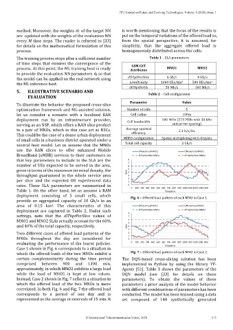
Two different cases of offered load patterns of the 2
MNOs throughout the day are considered for 1 0
evaluating the performance of the learnt policies. 0 100 200 300 400 500 600 700 800 900 1000 1100 1200 1300 1400
Time(min)
Case 1 shown in Fig. 6 corresponds to a situation in
which the offered loads of the two MNOs exhibit a Fig. 7 – Offered load pattern of each MNO in Case 2.
certain complementarity during the time period The DQN-based cross-slicing solution has been
comprised between 900 and 1300 min, implemented in Python by using the library TF-
approximately, in which MNO2 exhibits a large load Agents [51]. Table 3 shows the parameters of the
while the load of MNO1 is kept at low values. DQN model (see [33] for details on these
Instead, Case 2 shown in Fig. 7 reflects a situation in parameters). To obtain the values of these
which the offered load of the two MNOs is more parameters a prior analysis of the model behavior
correlated. In both Fig. 6 and Fig. 7 the offered load with different combinations of parameters has been
corresponds to a period of one day and is conducted. The model has been trained using a data
represented as the average in intervals of 15 min. It set composed of 140 synthetically generated

© International Telecommunication Union, 2020 113