Page 34 - ITU KALEIDOSCOPE, ATLANTA 2019

2019 ITU Kaleidoscope Academic Conference

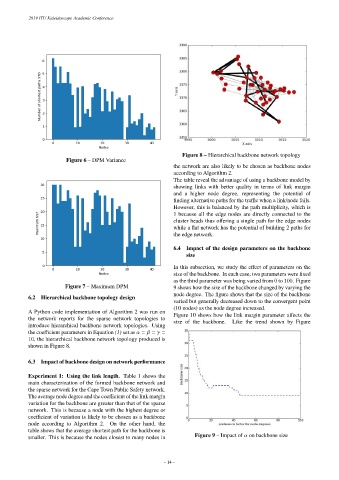
Figure 8 – Hierarchical backbone network topology
Figure 6 – DPM Variance
the network are also likely to be chosen as backbone nodes
according to Algorithm 2.
The table reveal the advantage of using a backbone model by
showing links with better quality in terms of link margin
and a higher node degree, representing the potential of
finding alternative paths for the traffic when a link/node fails.
However, this is balanced by the path multiplicity, which is
1 because all the edge nodes are directly connected to the
cluster heads thus offering a single path for the edge nodes
while a flat network has the potential of building 2 paths for
the edge network.

6.4 Impact of the design parameters on the backbone
size

In this subsection, we study the effect of parameters on the
size of the backbone. In each case, two parameters were fixed
as the third parameter was being varied from 0 to 100. Figure
Figure 7 – Maximum DPM 9 shows how the size of the backbone changed by varying the
node degree. The figure shows that the size of the backbone
6.2 Hierarchical backbone topology design
varied but generally decreased down to the convergent point
(10 nodes) as the node degree increased.
A Python code implementation of Algorithm 2 was run on Figure 10 shows how the link margin parameter affects the
the network reports for the sparse network topologies to size of the backbone. Like the trend shown by Figure
introduce hierarchical backbone network topologies. Using
the coefficient parameters in Equation (1) set as α = β = γ =
10, the hierarchical backbone network topology produced is
shown in Figure 8.

6.3 Impact of backbone design on network performance

Experiment 1: Using the link length. Table 1 shows the
main characterization of the formed backbone network and
the sparse network for the Cape Town Public Safety network.
The average node degree and the coefficient of the link margin
variation for the backbone are greater than that of the sparse
network. This is because a node with the highest degree or
coefficient of variation is likely to be chosen as a backbone
node according to Algorithm 2. On the other hand, the
table shows that the average shortest path for the backbone is
smaller. This is because the nodes closest to many nodes in Figure 9 – Impact of α on backbone size

– 14 –