Page 31 - ITU KALEIDOSCOPE, ATLANTA 2019

ICT for Health: Networks, standards and innovation

links have bigger differences in link margins. Therefore,
to know which nodes are well connected, the link
margin of each node is considered as the coefficient
of variation corresponding to the link margins of all the
links connected to that node. For a node i, the coefficient
lm(i) of variation is calculated as follows:
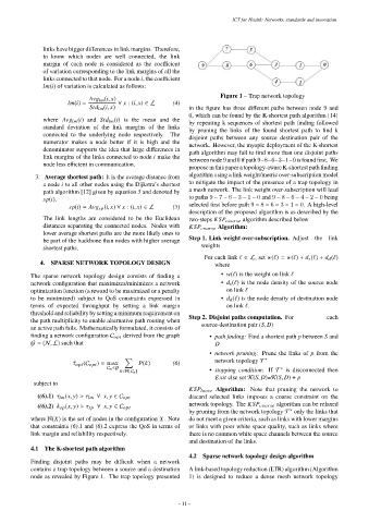
Figure 1 – Trap network topology
Avg lm (i, x)
lm(i) = ∀ x : (i, x) ∈ L (4)
Std lm (i, x) in the figure has three different paths between node 9 and
0, which can be found by the K-shortest path algorithm [14]
where Avg lm (i) and Std lm (i) is the mean and the by repeating k sequences of shortest path finding followed
standard deviation of the link margins of the links by pruning the links of the found shortest path to find k
connected to the underlying node respectively. The disjoint paths between any source destination pair of the
numerator makes a node better if it is high and the network. However, the myopic deployment of the K-shortest
denominator supports the idea that large differences in path algorithm may fail to find more than one disjoint paths
link margins of the links connected to node i make the between node 9 and 0 if path 9−8−6−3−1−0 is found first. We
node less efficient in communication. propose in this paper a topology-aware K-shortest path finding

3. Average shortest path: It is the average distance from algorithm using a link weight/metric over-subscription model
a node i to all other nodes using the Dijkstra’s shortest to mitigate the impact of the presence of a trap topology in
path algorithm [12] given by equation 5 and denoted by a mesh network. The link weight over-subscription will lead
sp(i). to paths 9 − 7 − 6 − 3 − 1 − 0 and 9 − 8 − 6 − 4 − 2 − 0 being
sp(i) = Avg sp (i, x) ∀ x : (i, x) ∈ L (5) selected first before path 9 − 8 − 6 − 3 − 1 − 0. A high-level
description of the proposed algorithm is as described by the
The link lengths are considered to be the Euclidean two-steps KSP coarse algorithm described below
distances separating the connected nodes. Nodes with KSP coarse Algorithm:
lower average shortest paths are the more likely ones to
be part of the backbone than nodes with higher average Step 1. Link weight over-subscription. Adjust the link
shortest paths. weights
For each link ` ∈ L, set w(`) = w(`) + d s (`) + d d (`)
4. SPARSE NETWORK TOPOLOGY DESIGN where

The sparse network topology design consists of finding a • w(`) is the weight on link `
network configuration that maximizes/minimizes a network • d s (`) is the node density of the source node
optimization function (a reward to be maximized or a penalty on link `
to be minimized) subject to QoS constraints expressed in • d d (`) is the node density of destination node
terms of expected throughput by setting a link margin on link `.
threshold and reliability by setting a minimum requirement on
the path multiplicity to enable alternative path routing when Step 2. Disjoint paths computation. For each
an active path fails. Mathematically formulated, it consists of source-destination pair (S, D)
finding a network configuration C opt derived from the graph • path finding: Find a shortest path p between S and
G = (N,L) such that D
• network pruning: Prune the links of p from the
Õ network topology T ∗
ˆ τ opt (C opt ) = max P(k) (6)
C n ∈G • stopping condition: If T is disconnected then
∗
k∈N[C n ]
Exit else set K(S, D)=K(S, D) + p
subject to
KSP loose Algorithm: Note that pruning the network to
discard selected links imposes a coarse constraint on the
((6).1) τ lm (x, y) > τ lm ∀ x, y ∈ C opt
network topology. The KSP coarse algorithm can be relaxed
((6).2) k sp (x, y) > τ sp ∀ x, y ∈ C opt
by pruning from the network topology T only the links that
∗
where N(X) is the set of nodes in the configuration X. Note do not meet a given criteria, such as links with lower margins
that constraints (6).1 and (6).2 express the QoS in terms of or links with poor white space quality, such as links where
link margin and reliability respectively. there is no common white space channels between the source
and destination of the links.
4.1 The K-shortest path algorithm
4.2 Sparse network topology design algorithm
Finding disjoint paths may be difficult when a network
contains a trap topology between a source and a destination A link-based topology reduction (LTR) algorithm (Algorithm
node as revealed by Figure 1. The trap topology presented 1) is designed to reduce a dense mesh network topology

– 11 –