Page 33 - ITU KALEIDOSCOPE, ATLANTA 2019

ICT for Health: Networks, standards and innovation

applied to map the targeted dense mesh network into a sparse
network. The final step of the network engineering process
consists of deriving a hierarchical backbone-based topology
as a topology that may be more scalable than the flat sparse
network topology.
The public safety mesh network design connecting police
stations in the city of Cape Town in South Africa depicted
in Figure 3 was used. The network design was simulated in
TV white space frequency using the Radio Mobile network
planning tool [15]. 42 network nodes were considered in the
simulation.
A Python code implementation of the LTR Algorithm 1 was
run on the network reports generated by the Radio Mobile
network planning tool [15] to map the dense mesh network
into sparse network topology. First, the GPS coordinates
of the nodes were transformed into 2-dimensional Cartesian
coordinates, which were used to compute Euclidean distances
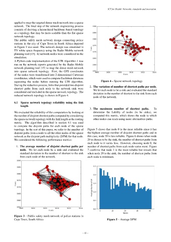
separating the nodes before running the LTR algorithm. Figure 4 – Sparse network topology
During the reduction process, links that provided two disjoint
shortest paths from each node to the network sink were 2. The variation of number of shortest paths per node.
We let each node to be a sink and evaluated the standard
considered and included in the sparse network topology. The deviation in the number of shortest to the sink from each
reduced network topology is shown in Figure 4. node of the network.

6.1 Sparse network topology reliability using the link
length
3. The maximum number of shortest paths. To
We evaluated the reliability of the computation by looking at determine the liability of nodes (to be sinks), we
the number of disjoint shortest paths computed by considering computed this metric, which shows the node to which
the sparse network topology with the link length as the routing other nodes can reach using more alternatives paths.
metric. The algorithm described in section 4.1 was used
to compute the disjoint paths for each node of the sparse
topology. In the rest of this paper, we refer to the number of Figure 5 shows that node 0 is the most reliable since it has
disjoint paths from a node to all the other nodes of the sparse the highest average number of disjoint shortest paths and in
network as the disjoint path multiplicity (DPM) for that node. this case, node 29 is less reliable. Figure 6 shows when node
We considered the following performance metrics: 29 is chosen to be the sink, the number of shortest paths from
each node to it varies less. However, choosing node 0, the
1. The average number of disjoint shortest paths per number of shortest paths from each node varies most. Figure
node. We let each node be a sink and evaluated the 7 confirms that node 1 is the most reliable but reveals that
standard deviation in the number of shortest to the sink when node 29 is the sink, the number of shortest paths from
from each node of the network. each node is minimum.

Figure 3 – Public safety mesh network of police stations in
Cape Town, South Africa Figure 5 – Average DPM

– 13 –