Page 55 - Proceedings of the 2018 ITU Kaleidoscope

Machine learning for a 5G future

= ( ) = / ( ). augmented intelligence, Case-Based Reasoning (CBR) and

The anomaly value components, one for each profile active learning methods to dynamically build and maintain a
centroid, are then aggregated in the following way. diagnosis knowledgebase, which can be utilized for both,
autonomous self-healing actions as well as supporting a
Let us denote the number of profile centroids and = human expert troubleshooting a network issue.

, ∈ {1, … , }, the distance vector of the observed

KPI-pair, , from the th profile centroid. The Euclidean 5.1 Diagnosis with case-based reasoning
distance is then calculated as = | |, ∈ {1, … , } among

which the closest one is determined as min =min . First, the detected anomaly events are described for

∈{ ,…, } diagnosis with an anomaly pattern. The anomaly pattern can
consist of the features (KPIs) used in the detection phase, but
Using the lengths = | |, ∈ {1, … , } of the anomaly typically it is an extension of these. As a medical analogy,

components, the resultant per KPI anomaly value is the fever is a good indicator of an illness, but for a diagnosing
weighted sum which illness it is, more information is required. In our
implementation, the averaged anomaly levels of an extended
∑ set of network KPIs were used. The anomaly pattern should
= ,
∑ capture as many aspects of the anomaly event as possible.

min
=e min ∀ ∈ {1, … , }, = 0.5 Next, the observed anomaly pattern is compared against the

already analyzed and labelled anomalies stored in the
4.3 Anomaly Event Detection diagnosis knowledgebase. The closest matching labelled
anomaly pattern or patterns are found, in the sense of
The goal of the anomaly event detection is to detect, as the similarity, and given as the most likely automated diagnosis.
name implies, distinct anomalies, which belong to the same Different distance measures were tested and in the end a
underlying event, based on the anomaly level timeseries combination of Euclidean and cosine distances was used.
values of the profiled features. First, for each profiled feature The distance measure gives the probability of the diagnosis.
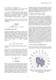
or KPI, anomalous timespans are detected using the Figure 3 depicts two anomaly patterns as a radar chart. Each
DBSCAN algorithm. An observation for feature k at time segment of the chart corresponds to a diagnosis feature. The
is considered anomalous if the anomaly value density outer blue area is the observed anomaly event and the inner
( ) goes above a given threshold orange area is the closest matching labelled anomaly in the

MinPts, . .: knowledgebase. The darker innermost circle is the expected
value for each feature and the actual observation can of
course be either above or below it.
( ) = | ( )| MinPts.

5.2 Active learning in the diagnosis process
, where is time window, in which the anomaly density is
calculated. Such CBR-based diagnosis function allows the diagnosis
knowledgebase to be developed and expanded dynamically
The start time of the anomaly comes from the above
,
definition, i.e. it is when the anomaly density exceeds the
threshold set by the MinPts. All subsequent points until end
of event , , where the density remains above it are
considered as part of the same event. The severity value of
the anomaly, for quantification purposes, is calculated as

, = ( ).

, ,
5 DIAGNOSIS

There is a vast diversity in the possible fault states that may
occur in a complex system like a mobile network. Therefore,
many of the fault states can be exceedingly rare. The lack of
statistical samples makes the reliable automated analysis of
the faults and the finding of the corrective actions extremely
difficult. And since we want to prepare also for the
unexpected and unprecedented, we need to combine machine Figure 3 – An anomaly pattern for an observed anomaly
learning with insights and the intuition of a human expert. event compared against a label in the diagnosis
We’ve developed a diagnosis concept, where we use knowledgebase

– 39 –