Page 54 - Proceedings of the 2018 ITU Kaleidoscope

2018 ITU Kaleidoscope Academic Conference

70.0k
1.40
60.0k
1.20
50.0k 1.00
800m
40.0k
600m
30.0k
400m

20.0k 200m
0.00
10.0k
-200m
0.00
-400m
0.00 2.00 4.00 6.00 8.00 10.0 12.0 14.0 16.0 18.0 20.0 22.0 0.00 20.0 40.0 60.0 80.0 100 120 140 160 180 200 220
Hour of day Average number of RRC connected UEs [#]

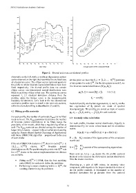
Figure 2 – Diurnal and cross-correlational profiles
observable on the left, while a nonlinear dependency pattern
can be observed on the right that resembles the enclosed area At this point we have the , ∈ 1,2,…, partitions

of a hysteresis curve. The ellipse curves represent quanta in of data points for each . For the data points in each we

the profile to which bivariate normal distributions have been fit a bivariate normal distribution ( , ):
fitted respectively. The diurnal profile does not contain
ellipse curves: one-dimensional normal distributions were
fitted to each hour of day in that case. The continuous curves 1, =mean :, , ∈ {1,2}

represent 1, 2.5 standard deviations distance from the
profiles, while the thicker curve is the parameterizable =cov( )

boundary for detection. Let’s look at the two-dimensional
correlation profiles more in detail in the next sub-sections, Vectors and are the two eigenvectors, and are the

while the diurnal profiling is described in [7] and [9]. two eigenvalues of (which are result of spectral

decomposition). The profiles are stored as triple of vectors
4.1 Fitting profile centroids , = and = for each centroid.

) to be fitted
For each profile, the number of centroids ( 4.2 Anomaly value calculation
needs to be set. The parameter determines the number
of bivariate normal distributions to be fitted, hence the For each profile, bivariate normal distribution, ( , ), is
granularity of the model, which has a regularizing effect as characterized by its vector valued mean and its covariance
well. The centroids are divided among the number of matrix.
larger initial clusters – created in the so-called pre-clustering
using the Density-Based Spatial Clustering of Applications ( , ) = + (0, ) = + (0, )
with Noise (DBSCAN) algorithm – proportional to the area
of each cluster. = ( ) consists of the eigenvectors of the covariance

matrix and
If the set of DBSCAN clusters is , then for each , ∈
{1, 2, …, | |} cluster, bivariate normal = consists of the corresponding eigenvalues
distributions are fit. For partitioning the points into sets
for a cluster in the current implementation two choices
are available: From now on, let = denote the th profile centroid

identical to the mean of the th bivariate normal distribution
• Fitting an ×1 SOM, then the best matching fit to the cluster members.
units (BMU) for each node define the partitions.
• Performing k-means clustering with = , the Observing , a pair of KPI values, its anomaly value
component, with regards to the largest standard deviation of
resulting clusters being the partitions
the th profile centroid, is determined as the number of
standard deviations the deviates from the centroid

– 38 –