Page 361 - Kaleidoscope Academic Conference Proceedings 2024

Innovation and Digital Transformation for a Sustainable World

CSV file for each individual image. Each CSV file is then Figure 6– Model Description
combined into a single file, for each folder (pose) given. A
function named ‘class_names’ is used to return the names of 11. CONFUSION MATRIX AND RESULT
the classes (poses). A final function named VISUALIZATION
‘all_landmarks_as_dataframe’ is used to combine all CSV
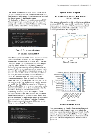
files corresponding to poses, into a single data frame. The After training and compilation, this model gives a validation
training data set CSV is split into Validation and Training accuracy of 0.87. The same model, when fit on the Testing
datasets, with the ratio of 3:17, to train the model. data set, gives an accuracy of 0.86. We also calculated and
plotted a Confusion Matrix to visualize the correct and
incorrect predictions in the Testing Dataset.

Figure 5– Pre-process code snippet
10. MODEL DESCRIPTION

After data augmentation in CSV format, need to convert the
data into tensors for the model. We first computed the
various centre points relevant to the pose, using a function Figure 7– Accuracy
‘get_center_point’. Our next step was to get a normalized
pose size. This is achieved by calculating distances of
landmarks from various centre points, and then taking an
average. Finally, the average is normalized to determine the
pose size. The landmarks are normalized depending on the
pose size. Since each landmark is denoted by coordinates
and score, the Input size initially is 51 (17 * 3) for our
model. We embed the input size, by expanding first,
normalizing landmarks based on coordinates, and then
flatten it to a size of 34. Due to this, our final input size for
the model is 34 (17 * 2). We introduced 3 hidden layers to
our model. Our first hidden layer consists of 128 neurons.
In the second and third layer, we go on reducing the number
of neurons by half the size of the previous layer. Thus the
second and third layers have 64 and 32 neurons,
respectively. At each layer, we are using ReLU as an
activation function. Along with the layers, we have added
Batch Normalization after each hidden layer. This is done
with the intention of normalizing the outputs of each hidden
layer, and tackling the problem of Vanishing Gradients.
This approach ensures that we can avoid the case of over-
fitting for various Yoga Pose Datasets
Figure 6– Confusion Matrix

As an extra measure to visualize the correct and incorrect
predictions, we added separate codes to investigate the
correct and incorrect predictions. The separation is done by
comparing y_true and y_predicted labels. For the images,
where the labels don’t match, they are shown as incorrect
predictions. The remaining images are shown as correct
predictions.

– 317 –