Page 111 - ITUJournal Future and evolving technologies Volume 2 (2021), Issue 1

ITU Journal on Future and Evolving Technologies, Volume 2 (2021), Issue 1

Table 5 – Example route matrix .
Energy Money Bit rate Hops
Sigfox BS 12 102 22 1
NB‐IoT BS 151 87 174 1
Node E (LoRa) 49 102 94 2
Table 6 – Requirements vectors.

Energy Money Bit rate
0.6 0.3 0.1
0.1 0.1 0.8
can forward its data to or using LoRa. The

latter can then of load ’s data to a base station with a

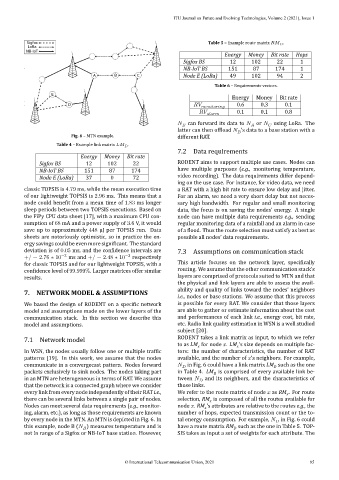
Fig. 6 – MTN example. different RAT.
Table 4 – Example link matrix .
7.2 Data requirements
Energy Money Bit rate
Sigfox BS 12 102 22 RODENT aims to support multiple use cases. Nodes can
NB‐IoT BS 151 87 174 have multiple purposes (e.g., monitoring temperature,
Node E (LoRa) 37 0 72 video recording). The data requirements differ depend‐
ing on the use case. For instance, for video data, we need
classic TOPSIS is 4.79 ms, while the mean execution time a RAT with a high bit rate to ensure low delay and jitter.
of our lightweight TOPSIS is 2.96 ms. This means that a For an alarm, we need a very short delay but not neces‐
node could bene it from a mean time of 1.83 ms longer sary high bandwidth. For regular and small monitoring
sleep periods between two TOPSIS executions. Based on data, the focus is on saving the nodes’ energy. A single
the FiPy CPU data sheet [17], with a maximum CPU con‐ node can have multiple data requirements e.g., sending
sumption of 68 mA and a power supply of 3.6 V, it would regular monitoring data of a rainfall and an alarm in case
save up to approximately 448 µJ per TOPSIS run. Data of a lood. Thus the route selection must satisfy as best as
sheets are notoriously optimistic, so in practice the en‐ possible all nodes’ data requirements.
ergy savings could be even more signi icant. The standard
deviation is of 0.05 ms, and the con idence intervals are 7.3 Assumptions on communication stack
+/ − 2.76 ∗ 10 −3 ms and +/ − 2.48 ∗ 10 −3 respectively
for classic TOPSIS and for our lightweight TOPSIS, with a This article focuses on the network layer, speci ically
con idence level of 99.999%. Larger matrices offer similar routing. We assume that the other communication stack’s
results. layers are comprised of protocols suited to MTN and that
the physical and link layers are able to assess the avail‐
ability and quality of links toward the nodes’ neighbors
7. NETWORK MODEL & ASSUMPTIONS
i.e., nodes or base stations. We assume that this process
We based the design of RODENT on a speci ic network is possible for every RAT. We consider that those layers
model and assumptions made on the lower layers of the are able to gather or estimate information about the cost
communication stack. In this section we describe this and performances of each link i.e., energy cost, bit rate,
model and assumptions. etc. Radio link quality estimation in WSN is a well studied
subject [20].
7.1 Network model RODENT takes a link matrix as input, to which we refer
to as LM for node . LM ’s size depends on multiple fac‐
x
x
In WSN, the nodes usually follow one or multiple traf ic tors: the number of characteristics, the number of RAT
patterns [19]. In this work, we assume that the nodes available, and the number of ’s neighbors. For example,
communicate in a convergecast pattern. Nodes forward in Fig. 6 could have a link matrix LM such as the one
D

packets exclusively to sink nodes. The nodes taking part in Table 4. LM is comprised of every available link be‐
D
in an MTN are heterogeneous in terms of RAT. We assume tween and its neighbors, and the characteristics of
that the network is a connected graph where we consider those links.
every link from every node independently of their RAT i.e., We refer to the route matrix of node as RM . For route
x
there can be several links between a single pair of nodes. selection, RM is composed of all the routes available for
x
Nodes can meet several data requirements (e.g., monitor‐ node . RM ’s attributes are relative to the routes e.g., the
x
ing, alarm, etc.), as long as those requirements are known number of hops, expected transmission count or the to‐
by every node in the MTN. An MTN is depicted in Fig. 6. In tal energy consumption. For example, in Fig. 6 could

this example, node B ( ) measures temperature and is have a route matrix RM such as the one in Table 5. TOP‐

D
not in range of a Sigfox or NB‐IoT base station. However, SIS takes as input a set of weights for each attribute. The
© International Telecommunication Union, 2021 95