Page 120 - ITU Journal Future and evolving technologies Volume 2 (2021), Issue 4 – AI and machine learning solutions in 5G and future networks

ITU Journal on Future and Evolving Technologies, Volume 2 (2021), Issue 4

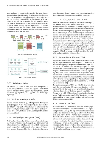
abnormal data entries to derive metrics that have changed puts the output through a nonlinear activation function.
since a failure, the differential data between the abnormal The mathematical representation of MLP output is:
data and normal data is used as input features. After that,

we can get three types of iles in the data set, which are = (Σ + ) = ( + )
=1

physical, virtual, and networks. To train a uni ied model
where is the vector of weights, is the vector of inputs,
for diverse network events, we merge all data sets into
is the bias, and is the activation function.
one CSV ile for putting into ML algorithms. The process
As a neural network based model, the MLP algorithm is a
is shown in Fig. 4. Finally, the data set for training consists
general function approximation method that can it com‑
of 930 lines with 996 features, and for evaluation consists
of 840 lines with 996 features. plex functions and adequately approximate complex non‑
linear relationships. It has a wide range of applications
and has features of high accuracy. It is often used to solve
classi ication problems. However, neural networks re‑
quire manual determination of a large number of param‑
eters, such as network topology, initial values of weights,
and thresholds. Learning may be not suf icient when the
parameter selection is inappropriate, and it is easy to fall
into local extremes. Besides, since MLP is a black‑box pro‑
cess, the learning process cannot be observed, and the
output is dif icult to interpret, which can affect the credi‑
bility and acceptability of the results.
Fig. 3 – Data differential method
3.2.2 Support Vector Machine (SVM)
Support Vector Machine (SVM) is a linear machine work‑
ing in a high dimensional feature space. SVM employs a
nonlinear mapping to map the ‑dimensional input vec‑
tor into a ‑dimensional feature space ( > ). The
problem that SVM tries to solve is to ind an optimal hy‑
perplane that correctly classi ies data points by separat‑
ing the points of two classes as much as possible. Both
classi ication and regression tasks transform the learn‑
ing task into a quadratic problem, but the way of creating
Fig. 4 – Data merging method
SVM networks varies depending on the classi ication and
regression tasks [19,20]. Excellent introductions to SVM
3.1.3 Label description can be found in [21].
The main advantages of SVM are (1) able to work with
As shown in Table 2, we have ive categories of high‑dimensional data; (2) high generalization perfor‑
labels for prediction, which are Type1: node‑down, mance without the need to add prior knowledge, even
Type3: interface‑down, Type57: tap‑loss (delay), Type9: when the dimension of the input space is very high.
ixnetwork‑bgp‑injection, and Type11: ixnetwork‑bgp‑ Compared to MLP, SVM performs better in classi ication
hijacking. mode. And in regression mode, MLP has better general‑
ization ability. In most cases, the observed performance
3.2 Machine learning methods difference is negligible [22].

In the related work in [4], Multiplelayer Perceptron 3.2.3 Decision Tree (DT)
(MLP), Support Vector Machine (SVM), and Random For‑
est (RF) are employed. In this study, as an extension of the A decision tree is a supervised machine learning algo‑
related work, three other kinds of tree‑based models, De‑ rithmthatcanbeappliedtobothclassi icationandregres‑
cision Tree (DT), XGBoost (XGB), and LightGBM(LGBM) sion problems. Usually, it is top‑down tree‑like structures
are also utilized. that explain the decision‑making rules for prediction. The
node from where the tree starts is known as a root node.
3.2.1 Multiplelayer Perceptron (MLP) The node where the tree ends is called the leaf node. Each
internal node can have two or more branches. A node rep‑
MLP is a feed‑forward arti icial neural network that maps resents a particular characteristic, while a branch repre‑
input data to the appropriate output. An MLP is a network sents a range of values. These ranges of values act as par‑
of simple neurons called a perceptron which computes a tition points for the set of values of the given characteris‑
single output from multiple real‑valued inputs. A Percep‑ tic. In Fig. 5, we provide an illustration of a decision tree,
tron forms a linear combination to its input weights and which is also used in our experiments:

104 © International Telecommunication Union, 2021