Page 96 - ITU Journal Future and evolving technologies Volume 2 (2021), Issue 1

ITU Journal on Future and Evolving Technologies, Volume 2 (2021), Issue 1

The number of redundancy bits are generated using the 10 0
following formula:

2 = + + 1, (2)
-2
where, represents the number of redundancy bits and 10
the number of information data bits. Hamming CR
1
For example, if we calculate the number of redundancy BER Fit Hamming CR
bits for a = 11 bits then it comes to add = 4 redun‑ Hamming CR 1
dancy bits. These parity/redundancy bits ( , , , ) 10 -4 Fit Hamming CR
2
8
1
2
4
are added to the information bits ( , ..., ) at the Hamming CR 2
1
11
transmitter (Hamming encoder) and then removed at the 4
Fit Hamming CR
receiver (Hamming decoder) which is able to detect and 4
correct errors. 10 -6
0 2 4 6 8 10 12
Bit po‑ E /N (dB)
b
0
sition 1 2 3 4 5 6 7 8 9 10 11 12 13 14 15
Encoded Fig. 3 – BER performance of the Hamming code for different coding rates
data 1 2 1 4 2 3 4 8 5 6 7 8 9 10 11 1 , 2 , 4
bits
frequently we have = 2 to use them as binary codes,
x x x x x x x x
1
2 x x x x x x x x each element being represented as a binary m‑tuple.
x x x x x x x x x
4 In terms of complexity, the Reed–Solomon encoder is
x x x x x x x x
fairly simple in terms of blocks and only involves multipli‑
8
Table 2 – The encoded bits for Hamming code [15, 11] ers and adders in the Galois Field. We can either create a
multiplication module or use RAM slots and create multi‑
TheHamming encoder calculatesthese parity bits accord‑ plication tables, However, the Reed–Solomon decoder in‑
ing to Table 2, and outputs a 15 bits message. The Ham‑ cludes several algorithms that consume a lot in resources,
ming Decoder calculates the parity bits: especially the Berlekamp algorithm.
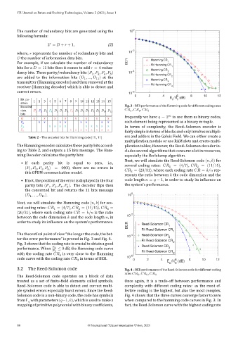
Next, we will simulate the Reed‑Solomon code ( , ) for
• If each parity bit is equal to zero, i.e., several coding rates: = (4/7), = (11/15),
1
2
( , , , ) = 0000, there are no errors in = (23/31), where each coding rate = / rep‑
2
4
1
8
this OFDM communication model. 3
resents the ratio between the code dimension and the
• If not, the position of the error is displayed in the four code length = − 1, in order to study its in luence on
parity bits ( , , , ). The decoder lips then the system’s performance.
1
8
2
4
the concerned bit and returns the 11 bits message
( , ..., ). 10 0
11
1
Next, we will simulate the Hamming code [ , ] for sev‑
eral coding rates: = (4/7), = (11/15), =
4
2
1
(26/31), where each coding rate = / is the ratio -2
between the code dimension and the code length , in 10
order to study its in luence on the system’s performance.
BER Reed-Solomon CR 1
Fit Reed-Solomon CR
1
The theoretical point of view “the longer the code, the bet‑ 10 -4 Reed-Solomon CR
ter the error performance” is proved in Fig. 3 and Fig. 4. 2
Fit Reed-Solomon CR
Fig. 3 shows that the coding rate is crucial to obtain a good Reed-Solomon CR 2
performance. When ≤ 9 dB, the Hamming code curve 3
0 Fit Reed-Solomon CR
with the coding rate is very close to the Hamming -6 3
4
code curve with the coding rate in terms of BER. 10 0 2 4 6 8 10 12
2
E /N (dB)
b 0
3.2 The Reed‑Solomon code Fig. 4 – BER performance of the Reed‑Solomon code for different coding
rates 1 , 2 , 3
The Reed‑Solomon code operates on a block of data
treated as a set of inite‑ ield elements called symbols. Once again, it is a trade‑off between performance and
Reed–Solomon code is able to detect and correct multi‑ complexity with different coding rates: as the most ef‑
ple symbol errors especially burst errors. Since the Reed‑ fective coding is the highest, but also the most complex.
Solomon code is a non‑binary code, the code has symbols Fig. 4 shows that the three curves converge faster to zero
from withparameters( −1, ), whichisusedtomakea when compared to the hamming code curves in Fig. 3. In

mapping of primitive polynomial with binary coef icients, fact, the Reed‑Solomon curve with the highest coding rate
80 © International Telecommunication Union, 2021