Page 104 - ITU Journal, Future and evolving technologies - Volume 1 (2020), Issue 1, Inaugural issue

ITU Journal on Future and Evolving Technologies, Volume 1 (2020), Issue 1

Table 2 – Simulation Parameters

Parameter Value
57 dBm
75 MHz
5.3 GHz
[0, 200] m
(a) 6 dB
[25, 50, 75] km/h

receiver node. The term is defined as

10 ( ) = − + 10 ( /4), (15)
10 10
where is the Equivalent Isotropic Radiated Power
(b) and [m] is the wavelength and represents the shad-
owing margin. In order to compute , we consider the
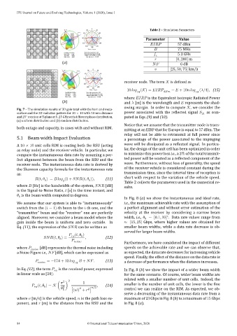
Fig. 7 – The simulation results of 3D gain total with the horn and meta-
surface and the 2D radiation pattern for 10 × 10 with 50 mm distance power associated with the reflected signal 21 as com-
∘
and25 rotationatY-planeat5.25GHzwithdifferentphasedistribution, puted in Eqs. (9) and (10).
(a) uniform distribution and (b) random distribution.
Notice that we assume that the transmitter node is trans-
both outage and capacity, in cases with and without RIM.
mitting at an EIRP that for Europe is equal to 57 dBm. The
relay will not be able to retransmit at full power since
5.1 Beam width Impact Evaluation a percentage of the power associated to the impinging
A 10 × 10 unit cells RIM is coating both the RSU (acting wave will be dissipated as a reflected signal. In particu-
as relay node) and the receiver vehicle. In particular, we lar, the design of the unit cell has been optimized in order
compute the instantaneous data rate by assuming a per- to minimize this power loss i.e., a 2% of the total transmit-
fect alignment between the beam from the RSU and the ted power will be wasted as a reflected component of the
receiver node. The instantaneous data rate is derived by wave. Furthermore, without loss of generality, the speed
the Shannon capacity formula for the instantaneous rate of the receiver vehicle is considered constant during the
as: transmission time, since the interval time of reception is
( , ) = (1 + ( , )), (11) short with respect to the variation of the vehicle speed.

2
Table 2 collects the parameters used in the numerical re-
where [Hz] is the bandwidth of the system, [dB]
sults.
is the Signal-to-Noise Ratio, [s] is the time instant, and
is the beam width computed in degrees.

In Fig. 8 (a) we show the instantaneous and ideal rate,
We assume that our system is able to “instantaneously” i.e., the maximum achievable rate with the assumption of
switch from the ( − 1)-th beam to the -th one, and the a perfect alignment and without error estimation of the
“transmitter” beam and the “receiver” one are perfectly velocity at the receiver by considering a narrow beam
∘
aligned. Moreover, we consider a beam model where the width, i.e., = [0.1, 10] . Data rate values range from

gain inside the beam is uniform and zero outside. In ≈ [15, 25] Gbps, where higher values are obtained for
Eq. (11), the expression of the can be written as smaller beam widths, while a data rate decrease is ob-
served for larger beam widths.
( , )
( , ) = , (12)

Furthermore, we have considered the impact of different
where [dB] represents the thermal noise including speeds on the achievable rate and we can observe that,
a Noise Figure i.e., [dB], which can be expressed as as expected, the data rate decreases for increasing vehicle
speed. Finally, the effect of the distance on the data rate is
= −174 + 10 10 + . (13) a decrease of performance when the distance increases.
In Eq. (12), the term is the received power, expressed In Fig. 8 (b) we show the impact of a wider beam width
in linear scale as [10]: for the same scenario. Of course, wider beam widths are
related with a smaller number of unit cells. Indeed, the
2
2 1
( , ) = ( ) , (14) smaller is the number of unit cells, the lower is the fine

2 [( ) + ] /2 control we can realize on the RIM. As expected, we ob-
2
2
serve a decreasing of the instantaneous data rate from a
where [m/s] is the vehicle speed, is the path loss ex- maximum of 23 Gbps in Fig. 8 (b) to a maximum of 15 Gbps
ponent, and [m] is the distance from the RSU and the in Fig. 8 (a).

84 © International Telecommunication Union, 2020