Page 58 - ITU Journal: Volume 2, No. 1 - Special issue - Propagation modelling for advanced future radio systems - Challenges for a congested radio spectrum

ITU Journal: ICT Discoveries, Vol. 2(1), December 2019

Table 5 – Simulation parameters ⋅10 −2
1
RTS
= 0.3
0.8 DACM
ITU-R urban parameters = 500 buildings/km 2

= 15
0.6
Virtual city side length ( ) 1600 m ( m )
BS height (ℎ ) 30 m 0.4
BS
MS height (ℎ ) 1.5 m
MS
Number of MS ( ) 3771 0.2
BS transmit power (P ) 20 dBm 0
t
Carrier frequency ( ) 2 GHz, 28 GHz −180 −135 −90 −45 0 45 90 135 180

Cut-off power (P ) -150 dBm (degree)
m
off
Max rays per MS (ℛ MAX ) 100 (a) = 2 GHz
Cluster gap ( ) 50 ∘
⋅10 −2
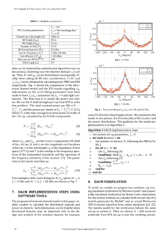
data can be clustered by sophisticated algorithms such as 1
RTS
hierarchical clustering once the shortest distance is set 0.8 DACM
up. Then ℳ and can be determined consequently. Fi-
m
nally when taking all MS into consideration, (ℳ) and 0.6
( ) can be obtained by calculating their PMF and PDF ( m )

m
respectively. Fig. 6 shows the comparison of the direc- 0.4
tional channel model and the RTS results regarding . 0.2
m
Adjustments on the curve itting parameters have been
0
made to have ( ) symmetric on = 0 and right con- −180 −135 −90 −45 0 45 90 135 180

m
m
tinuous. The inal step is to model the power per clus- (degree)
m
ter. We use the E- ield strength per ray from RTS to solve
this problem. The total received power per MS is P = (b) = 28 GHz
r
∑ ℛ , and the power per cluster is P = ∑ ℛ m [27], Fig. 6 – The curve itting of ( m ) at 2 GHz and 28 GHz.
=1 m =1
where is the time averaged received power in watts of

the -th ray, calculated by the E- ield components: some 5G direction-based applications. We summarize the
model in two phases, the directionality of the clusters and
the power distribution. The guideline for the model im-
2
2
= 8 0 ∣ , + , ∣ (8) plementation is in Algorithm 1.

2
2 Algorithm 1 DACM implementation steps
= ∣ , + , , ∣ . (9) 1: Get system set-up parameters, ,
,
8 0 2: for each Receiver do
where , and , are the and components of E- ield 3: Get number of clusters ℳ, following the PMF in Ta-
of the -th ray, and are the magnitude and the phase ble 2
of the ray, is the wavelength, is the impedance of free 4: for all m ∈ ℳ do
0
space (377 Ω) and is the overlap of the frequency spec- 5: Get following (4)
m
trum of the transmitted waveform and the spectrum of 6: Condition: MAX( − m-1 ) ≤ , m = 2...ℳ
m
the frequency selectivity of the receiver [27]. The power 7: Get following (7)
m
ratio in (6) can be rewritten as: Condition: ∑ ℳ = 1
8:
m=1 m
9: P ← P
2 m m r
∑ ℛ m ∣ , + , ∣ 10: end for
= =1 , , 2 . (10)
m
∑ ℛ ∣ , + , ∣ 11: end for
=1 , ,
Two examples of the curve itting for ( ) given ℳ = 2,
m
= 2 GHz and ℳ = 3, = 28 GHz are shown in Fig. 7. 8. DACM VERIFICATION

To verify our model, we propose two methods, ray trac-
®
7. DACM IMPLEMENTATION STEPS USING ing simulated veri ication by Wireless Insite and numer-
SOFTWARE TOOLS ically simulated veri ication by Monte-Carlo simulations.
For the former method, we consider both virtual city (VC)
The proposed directional channel model in this paper en- models generated by Matlab and an actual Melbourne
®
ables readers to calculate the distributed azimuth and CBD footprint imported from online databases [24, 25].
power in clusters. Such information can be helpful when The system model for the veri ication follows the same
directional features play an important role in the de- set-up as section 3. Then we choose = 500 receivers
sign and analysis of the wireless channel, for example, uniformly from RTS set-up to join the verifying calcula-
42 © International Telecommunication Union, 2019