Page 56 - ITU Journal: Volume 2, No. 1 - Special issue - Propagation modelling for advanced future radio systems - Challenges for a congested radio spectrum

ITU Journal: ICT Discoveries, Vol. 2(1), December 2019

for the result of and . It is common in the existing lit-
erature that the authors start analyzing the channel from
the delay domain, and the azimuth spread has some cor-
relation with the delay [8, 9]. In this paper, we believe
that it is worthy of focusing more on the features of the
directionality of the wireless channel.

Fig. 4 – The methodology of directional antenna channel modeling.
5. DIRECTIONAL ANTENNA CHANNEL
MODELING

In this section, we propose the directional antenna chan-
nel model. Firstly, we will introduce the clusters of the
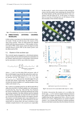
rays at the receiver. Then we will present the channel (a) Visualized clustered rays in the ray tracing simulator.
model with three key parameters: 1) the number of clus-
ters and its PMF; 2) the cluster center (in degrees) in the
azimuth domain and its PDF; 3) the cluster power ratio
(in dBm) and its PDF.

5.1 Clusters of the incident rays
The received signal propagated in a directional antenna
channel model can be characterized by the summation of
the clusters, and each cluster can be further characterized
by the summation of all the rays within the cluster:

ℳ ℛ m
( i, m , i, m , i, m ) = ∑ ∑ i, m ( i, m , i, m , i, m ) (2) (b) Clustered rays in the delay domain.
⏟⏟⏟⏟⏟⏟⏟⏟⏟⏟⏟
m=1 i=1
m ( i, m , i, m , i, m )
where , and are the delay, DOA and power ratio of
the received signal respectively, the subscript m and i rep-
resent the corresponding parameters of the m-th clus-
ter and the i-th ray. The terms i, m ( i, m , i, m , i, m ) and
( i, m , i, m , i, m ) represent the received signal of each
m
ray and each cluster, respectively. We de ine that at one
receiver, the cluster number is ℳ, and the number of rays
within each cluster is ℛ .
m
Fig. 5 shows an example given by one MS located 600 m (c) Clustered rays in the azimuth domain.
away from the BS in a virtual random city environment. Fig. 5 – An example of the rays in clusters with respect to and .
In particular, Fig. 5(a), Fig. 5(b) and Fig. 5(c) illustrate
the cluster classi ication considering clustered rays in the To further characterize the clusters of , we de ine the
ray tracing simulator, the delay domain and the azimuth cluster gap, , as the shortest angular distance between
DOA domain, respectively. As expected, the received rays two clusters in degree. In other words, if the DOA of two
are clustered in both delay domain and angular domain. neighboring rays has a gap greater than , these two rays
The clusters in both domains have some similarities to a fall into two clusters. Noting that in our system model in
certain degree. However, the cluster division in two do- section 3, we consider MS located at random positions.
mains does not always share the exact consistency since However, the inal results show that the distance between
multiple complex factors in the scenario are responsible

40 © International Telecommunication Union, 2019