Page 36 - ITU Journal: Volume 2, No. 1 - Special issue - Propagation modelling for advanced future radio systems - Challenges for a congested radio spectrum

ITU Journal: ICT Discoveries, Vol. 2(1), December 2019

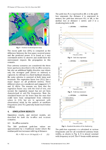
The path loss PL is expressed in dB; n is the path-
loss exponent; the distance d is expressed in
meters; the path-loss intersect PLI, in dB, is the
median loss at distance 1 meter; and S is a
shadowing term in dB.

Fig. 3 – Outdoor received power map
The excess path loss (EPL) is computed as the
difference between the free-space received power
and the predicted power. It is found as a very
convenient metric to observe and model how the Fig. 4 – Path-loss exponent
environment impacts the propagation in this
scenario.
Four antenna scenarios are considered: the three
beam apertures described in the in-office scenario,
but also an additional highly-directive case where
only the strongest path (direct or indirect) is
captured. As relevant in a fixed backhaul situation,
the same antenna is assumed at both lamp post
terminals. The vegetation linear loss (VLL) has a
major impact on all predicted metrics. Three
different values are considered, and compared: 6, 9
and 12 dB/m. The reasons are, first, that the
vegetation losses vary with the kind of tree, and
second, the vegetation impact has not yet been Fig. 5 – Path-loss intersect
characterized at sub-THz frequencies. Note the
simulated losses are far lower than the ones that
could have been extrapolated from reference
values in [13], but are in agreement with
observations made by the authors at mmWave
frequencies (tree VLL generally found much below
5 dB/m).

4. SIMULATION RESULTS

Simulation results, and derived models, are
described for both the in-office and in-street
scenarios.
4.1 In-office scenario

The 500 predicted path-loss values are Fig. 6 – Standard deviation of the shadowing
approximated by a traditional model where the The path-loss exponent n is calculated at various
median path loss increases with log of distance: frequencies and for all considered antenna beam

= + × 10 ( ) + (1) widths, as shown in Fig. 4. It is almost constant
with frequency in LoS. The 6°-beam-width antenna

20 © International Telecommunication Union, 2019