Page 27 - ITU Journal: Volume 2, No. 1 - Special issue - Propagation modelling for advanced future radio systems - Challenges for a congested radio spectrum

ITU Journal: ICT Discoveries, Vol. 2(1), December 2019

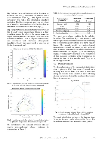
Fig. 2 shows the scintillation standard deviation at Table 2 – Correlation between scintillation standard deviation
Ka-band versus . As we can see, there is also a and meteorological parameters
clear correlation with ; the higher the wet Meteorological Correlation Correlation
refractivity the higher the scintillation standard parameter Ka-band Q-band
deviation. The parameter, averaged on a long
term basis, has been used to model the distribution Pressure (mB) −0.31 −0.29
of the scintillation standard deviation[5]–[7]. Nwet 0.33 0.34
Temperature (ºC) 0.34 0.36
Fig. 3 depicts the scintillation standard deviation at Water vapor (g/m ) 0.33 0.35
3
the Q-band versus temperature. There is a clear Relative humidity 0.14 0.12
trend that shows the effect of the temperature; the
higher the temperature the higher the scintillation The most uncorrelated variable is the relative
standard deviation. That is, higher temperatures humidity. The variables , temperature and
are associated with increased atmospheric water vapor content have similar correlations being
instability. Exactly the same trend is observed at the corresponding correlations at Q-band slightly
Ka-band (not depicted). higher. The models usually use meteorological
parameters averaged on longer periods as input
data, however, a noticeable correlation is observed
with hourly data. The Ortgies-T [8] and Marzano [9]
models seem to deserve attention as the correlation
of the standard deviation with temperature is
similar to that of the usually used as a
modeling parameter.

4.2 Diurnal variation
The diurnal variation of the standard deviation (the
time is given in UTC) has been calculated on a
monthly and yearly basis. The trend is the same
along all months with somewhat more striking
diurnal variations during the months with average
higher temperatures.

Fig. 2 – Joint histogram (in log.units) of the standard deviation
at Ka-band vs Nwet; the contours are log spaced

Fig. 4 – Hourly average values of the scintillation standard
deviation at the Q and Ka bands in August 2017
The most scintillating periods of the day are from
Fig. 3 – Joint histogram (in log units) of the standard deviation 10 am to 8 pm as can be observed in Fig. 4; this
at Q-band vs temperature; the contours are log spaced latter hour occurs a little bit earlier during winter.
The correlation of the standard deviation with the
several meteorological related variables is
summarized in Table 2.

© International Telecommunication Union, 2019 11